Please solve for distance and field strength data to fit within the code arrays. In the Appendix there are two images. Each is of one of the two floors of a commercial building.

A $915-MHz$ transmitter was placed at the point marked TX on the first floor. The distance

between upper$-$most and lower$-$most walls $($the vertical building dimension along the $"x"$ axis$)$ is

$180$ feet. The distance between floors is $13$ feet. Measurements of received field strength at

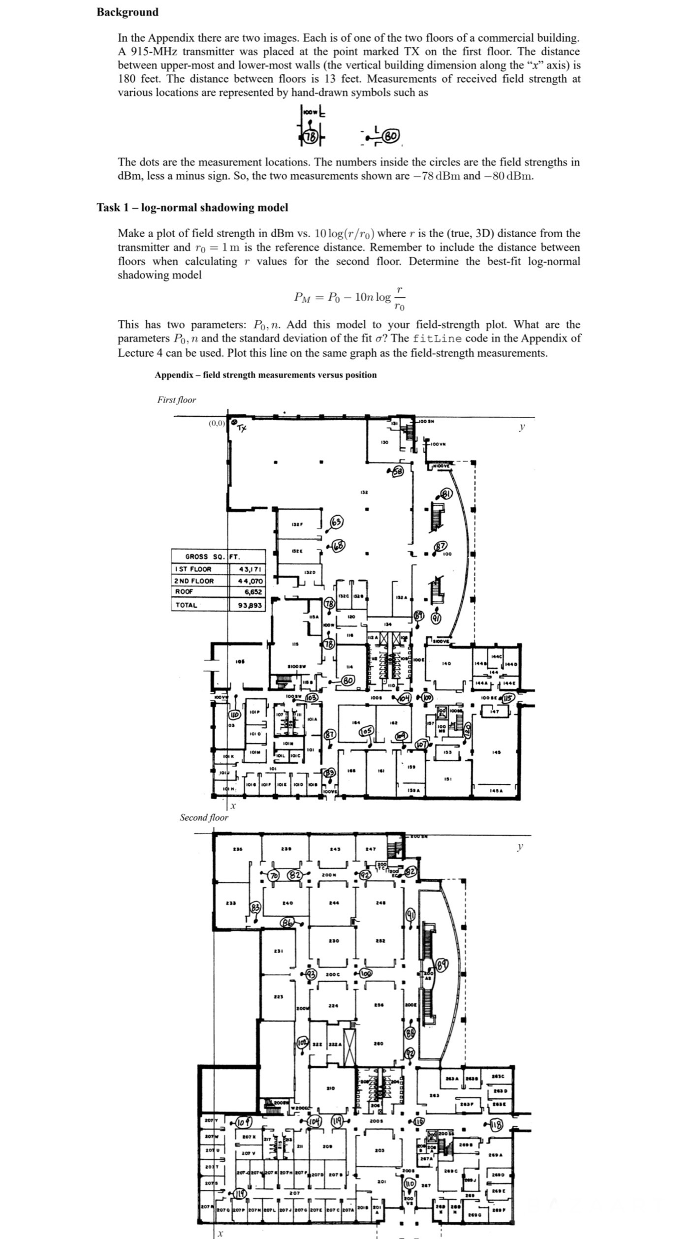
various locations are represented by hand$-$drawn symbols such as

$-\frac{1}{r}B0.$

The dots are the measurement locations. The numbers inside the circles are the field strengths in

$dBm,$ less a minus sign. So$,$ the two measurements shown are $-78dBm$ and $-80dBm.$

Task $1-$ log$-$normal shadowing model

Make a plot of field strength in $dBm$ vs$.10log(\frac{r}{r_0})$ where $r$ is the $($true$,3$D$)$ distance from the

transmitter and $r_0=1m$ is the reference distance. Remember to include the distance between

floors when calculating $r$ values for the second floor. Determine the best$-$fit log$-$normal

shadowing model

$P_M=P_0-10nlog\frac{r}{r_0}$

This has two parameters: $P_0,n.$ Add this model to your field$-$strength plot. What are the

parameters $P_0,n$ and the standard deviation of the fit $?$ The fitLine code in the Appendix of

Lecture $4$ can be used. Plot this line on the same graph as the field$-$strength measurements.

Appendix $-$ field strength measurements versus position

First floor

Second floor$\%$ Replace 'distance' and 'field$\_$strength' with your actual data

$\%$ Example:

x $=[1,2,3,4,5]$; $//$replace with your actual distance data

y $=[60,55,50,45,40]$; $//$replace with your actual field strength data$//$Fit log$-$normal shadowing model

$[$alpha$,$ beta, sigma$]=$ fitLogNormal$($x$,$ y$)$;

disp$(\text{'}$Log$-$Normal Shadowing Model Parameters:$\text{'})$;

disp$([\text{'}$Alpha $($intercept$)$: $\text{'}+$ string$($alpha$)])$;

disp$([\text{'}$Beta $($slope$)$: $\text{'}+$ string$($beta$)])$;

disp$([\text{'}$Sigma $($standard deviation$)$: $\text{'}+$ string$($sigma$)])$;

$//$Plot the field strength data

plot$($x$,$ y$,\text{'}$o$\text{'},$ 'MarkerSize', $10,$ 'MarkerFaceColor', $\text{'}$b$\text{'})$;

hold on;

$//$Generate log$-$normal shadowing model curve for plotting

x$\_$fit $=$ linspace$($min$($x$),$ max$($x$),100)$;

y$\_$fit $=$ alpha $+$ beta $*$ log$($x$\_$fit$)$;

plot$($x$\_$fit, y$\_$fit, $\text{'}$r$-\text{'},$ 'LineWidth', $2)$;

xlabel$(\text{'}$Distance$\text{'})$;

ylabel$(\text{'}$Field Strength $($dBm$)\text{'})$;

title$(\text{'}$Field Strength vs$.$ Distance with Log$-$Normal Shadowing Model'$)$;

legend$(\text{'}$Field Strength Data', 'Log$-$Normal Shadowing Model'$)$;

grid on;

hold off;