Please solve in R!

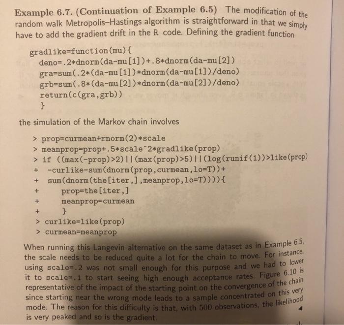
Exercise 6.7 Referring to Example 2.7, consider a Be(2.7,6.3) target density. a. Generate Metropolis-Hastings samples from this density using a range of indepen- dent beta candidates from a Be(1, 1) to a beta distribution with small variance. (Note: Recall that the variance is ab/(a + b) (a +6+1).) Compare the acceptance rates of the algorithms. b. Suppose that we want to generate a truncated beta Be(2.7,6.3) restricted to the interval (c,d) with c, d e (0,1). Compare the performance of a Metropolis- Hastings algorithm based on a Be(2,6) proposal with one based on a Ulc,d) pro- posal. Take c= .1,.25 and d= .9,.75. Example 6.7. (Continuation of Example 6.5) The modification of the random walk Metropolis-Hastings algorithm is straightforward in that we simply have to add the gradient drift in the R code. Defining the gradient function gradlike=function(mu) { deno= 2*dnorm(da-mu[1])+. 8*dnorm(da-mu[2]) gra=sum(.2*(da-mu [1]) *dnorm(da-mu[1])/deno) grb=sum(.8*(da-mu[2])*dnorm(da-mu[2])/deno) return(c(gra,grb)) } the simulation of the Markov chain involves + + + + + > prop=curmean+rnorm(2)*scale > meanprop=prop+.5*scale 2*gradlike(prop) > if ((max(-prop)>2)||(max(prop) >5)||(log(runif(1))>like (prop) -curlike-sum (dnorm(prop, curmean, lo=T))+ sum (dnorm(the[iter,),meanprop, lo=T)))) { prop=the [iter,] meanprop=curmean } > curlike-like (prop) > curmean=meanprop When running this Langevin alternative on the same dataset as in Example 6.5, the scale needs to be reduced quite a lot for the chain to move. For instance, using scale-2 was not small enough for this purpose and we had to lower it to scale-.1 to start seeing high enough acceptance rates. Figure 6.10.is representative of the impact of the starting point on the convergence of the chain since starting near the wrong mode leads to a sample concentrated on this very mode. The reason for this difficulty is that, with 500 observations, the likelihood is very peaked and so is the gradient. Exercise 6.7 Referring to Example 2.7, consider a Be(2.7,6.3) target density. a. Generate Metropolis-Hastings samples from this density using a range of indepen- dent beta candidates from a Be(1, 1) to a beta distribution with small variance. (Note: Recall that the variance is ab/(a + b) (a +6+1).) Compare the acceptance rates of the algorithms. b. Suppose that we want to generate a truncated beta Be(2.7,6.3) restricted to the interval (c,d) with c, d e (0,1). Compare the performance of a Metropolis- Hastings algorithm based on a Be(2,6) proposal with one based on a Ulc,d) pro- posal. Take c= .1,.25 and d= .9,.75. Example 6.7. (Continuation of Example 6.5) The modification of the random walk Metropolis-Hastings algorithm is straightforward in that we simply have to add the gradient drift in the R code. Defining the gradient function gradlike=function(mu) { deno= 2*dnorm(da-mu[1])+. 8*dnorm(da-mu[2]) gra=sum(.2*(da-mu [1]) *dnorm(da-mu[1])/deno) grb=sum(.8*(da-mu[2])*dnorm(da-mu[2])/deno) return(c(gra,grb)) } the simulation of the Markov chain involves + + + + + > prop=curmean+rnorm(2)*scale > meanprop=prop+.5*scale 2*gradlike(prop) > if ((max(-prop)>2)||(max(prop) >5)||(log(runif(1))>like (prop) -curlike-sum (dnorm(prop, curmean, lo=T))+ sum (dnorm(the[iter,),meanprop, lo=T)))) { prop=the [iter,] meanprop=curmean } > curlike-like (prop) > curmean=meanprop When running this Langevin alternative on the same dataset as in Example 6.5, the scale needs to be reduced quite a lot for the chain to move. For instance, using scale-2 was not small enough for this purpose and we had to lower it to scale-.1 to start seeing high enough acceptance rates. Figure 6.10.is representative of the impact of the starting point on the convergence of the chain since starting near the wrong mode leads to a sample concentrated on this very mode. The reason for this difficulty is that, with 500 observations, the likelihood is very peaked and so is the gradient