

Question: Please solve this using python. Please show the code and explain! The following code is the perceptron implementation from the textbook (with only three lines
Please solve this using python. Please show the code and explain!
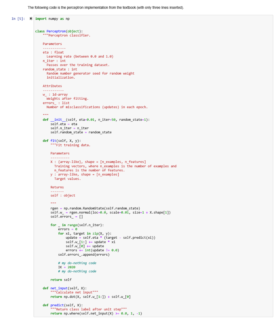
![three lines inserted). In [5]: Nimport numpy as np class Perceptron(object): **](https://s3.amazonaws.com/si.experts.images/answers/2024/07/66a6b33e38a12_89366a6b33dafa55.jpg)
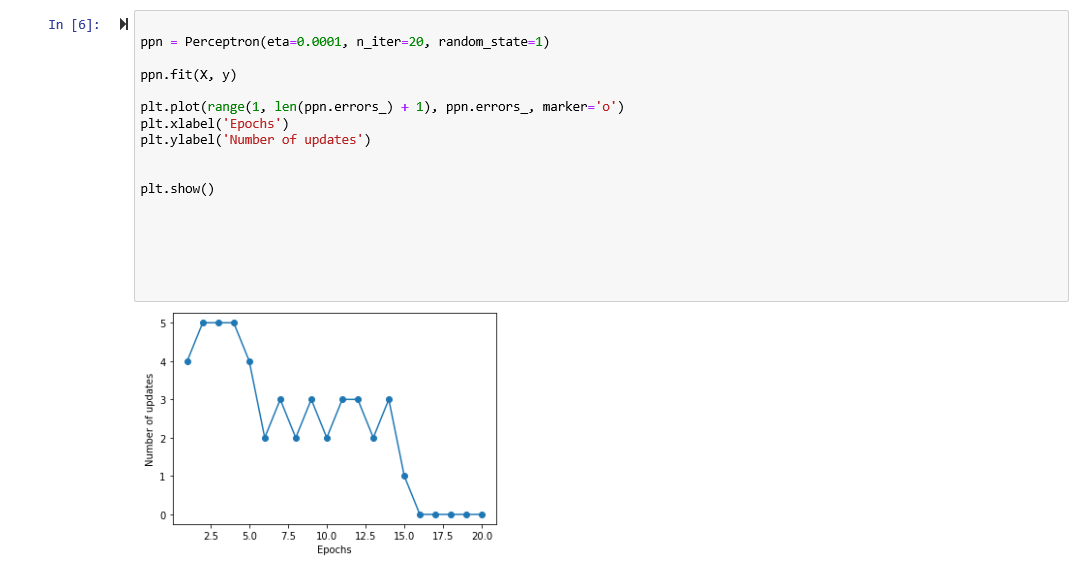
The following code is the perceptron implementation from the textbook (with only three lines inserted). In [5]: Nimport numpy as np class Perceptron(object): ** Perceptron classifier. Parameters eta : float Learning rate (between 0.2 and 1.0) n iter : int Passes over the training dataset. random_state : int Random number generator seed for random weight initialization. Attributes W 1d-array Weights after fitting. errors: list Number of misclassifications (updates) in each epoch. def __init__(self, eta=0.01, n_iter-50, random_state-1): self.eta - eta self.n_iter = niter self.random_state = random_state def fit(self, x, y): **Fit training data. Parameters X : {array-like), shape = [n_examples, n_features] Training vectors, where n_examples is the number of examples and n_features is the number of features. y : array-like, shape = [n_examples] Target values. Returns self : object rgen - np.random. RandomState(self.random_state) self.w = rgen.normal(loc-2.0, scale-0.01, size-1 + X.shape[1]) self.errors = [] for _ in range(self.n_iter): errors = 0 for xi, target in zip(x, y): update = self.eta * (target - self.predict(xi)) self.w_[1:] += update * xi self.w_[@] += update errors += int(update != 0.6) self.errors_.append(errors) # my do-nothing code IK = 2020 # my do-nothing code return self def net input(self, x): **"Calculate net input" return np.dot(X, self.w_[1:)) + self.w_[@] def predict(self, x): ***"Return class label after unit step""" return np.where(self.net_input(x) >= 0.0, 1, -1) In [6]: N ppn = Perceptron(eta=0.0001, n_iter=20, random_state=1) ppn.fit(x, y) plt.plot(range(1, len(ppn.errors_) + 1), ppn.errors, marker='0') plt.xlabel('Epochs') plt.ylabel('Number of updates') plt.show() Number of updates 25 50 75 10.0 12.5 Epochs 15.0 17.5 20.0 Question 3: Visualizing multiple decision regions over time Here is the function for visualizing decision regions In [7]: from matplotlib.colors import ListedColormap def plot_decision_regions(x, y, classifier, resolution=0.02): # setup marker generator and color map markers = ('s', 'x', 'o', 'A', 'v') colors = ('red', 'blue', 'lightgreen', 'gray', 'cyan') cmap = ListedColormap(colors[:len(np.unique(y)))) # plot the decision surface x1_min, x1_max = X[:, ].min() - 1, X[:, ].max() + 1 X2_min, X2_max = X[:, 1].min() - 1, X[:, 1].max() + 1 xx1, xx2 = np.meshgrid(np.arange (x1_min, x1_max, resolution), np.arange (x2_min, X2_max, resolution)) Z = classifier.predict(np.array([xxl.ravel(), xx2.ravel()]).T) Z = Z.reshape(xxl.shape) plt.contourf(xxl, xx2, Z, alpha=0.3, cmap=cmap) plt.xlim(xx1.min(), xx1.max()) plt.ylim(xx2.min(), Xx2.max()) # plot class examples for idx, cl in enumerate(np.unique(y)): plt. scatter(x=X[y == cl, ], y=X[y == cl, 1], alpha=0.8, C=colors[idx] marker=markers[idx), label=cl, edgecolor='black') In [8]: plot_decision_regions(x, y, classifier=ppn) plt.xlabel('sepal length [cm]') plt.ylabel('petal length [cm]') plt. legend(loc='upper left') # plt. savefig('images/02_08.png', dpi=300) plt.show() petal length (cm) sepal length (cm) Using the above, give code that plots the decision regions for the first 5 epochs. Use learning rate = 0.01 and random seed = 1 when applicable. In [9]: # The following code is the perceptron implementation from the textbook (with only three lines inserted). In [5]: Nimport numpy as np class Perceptron(object): ** Perceptron classifier. Parameters eta : float Learning rate (between 0.2 and 1.0) n iter : int Passes over the training dataset. random_state : int Random number generator seed for random weight initialization. Attributes W 1d-array Weights after fitting. errors: list Number of misclassifications (updates) in each epoch. def __init__(self, eta=0.01, n_iter-50, random_state-1): self.eta - eta self.n_iter = niter self.random_state = random_state def fit(self, x, y): **Fit training data. Parameters X : {array-like), shape = [n_examples, n_features] Training vectors, where n_examples is the number of examples and n_features is the number of features. y : array-like, shape = [n_examples] Target values. Returns self : object rgen - np.random. RandomState(self.random_state) self.w = rgen.normal(loc-2.0, scale-0.01, size-1 + X.shape[1]) self.errors = [] for _ in range(self.n_iter): errors = 0 for xi, target in zip(x, y): update = self.eta * (target - self.predict(xi)) self.w_[1:] += update * xi self.w_[@] += update errors += int(update != 0.6) self.errors_.append(errors) # my do-nothing code IK = 2020 # my do-nothing code return self def net input(self, x): **"Calculate net input" return np.dot(X, self.w_[1:)) + self.w_[@] def predict(self, x): ***"Return class label after unit step""" return np.where(self.net_input(x) >= 0.0, 1, -1) In [6]: N ppn = Perceptron(eta=0.0001, n_iter=20, random_state=1) ppn.fit(x, y) plt.plot(range(1, len(ppn.errors_) + 1), ppn.errors, marker='0') plt.xlabel('Epochs') plt.ylabel('Number of updates') plt.show() Number of updates 25 50 75 10.0 12.5 Epochs 15.0 17.5 20.0 Question 3: Visualizing multiple decision regions over time Here is the function for visualizing decision regions In [7]: from matplotlib.colors import ListedColormap def plot_decision_regions(x, y, classifier, resolution=0.02): # setup marker generator and color map markers = ('s', 'x', 'o', 'A', 'v') colors = ('red', 'blue', 'lightgreen', 'gray', 'cyan') cmap = ListedColormap(colors[:len(np.unique(y)))) # plot the decision surface x1_min, x1_max = X[:, ].min() - 1, X[:, ].max() + 1 X2_min, X2_max = X[:, 1].min() - 1, X[:, 1].max() + 1 xx1, xx2 = np.meshgrid(np.arange (x1_min, x1_max, resolution), np.arange (x2_min, X2_max, resolution)) Z = classifier.predict(np.array([xxl.ravel(), xx2.ravel()]).T) Z = Z.reshape(xxl.shape) plt.contourf(xxl, xx2, Z, alpha=0.3, cmap=cmap) plt.xlim(xx1.min(), xx1.max()) plt.ylim(xx2.min(), Xx2.max()) # plot class examples for idx, cl in enumerate(np.unique(y)): plt. scatter(x=X[y == cl, ], y=X[y == cl, 1], alpha=0.8, C=colors[idx] marker=markers[idx), label=cl, edgecolor='black') In [8]: plot_decision_regions(x, y, classifier=ppn) plt.xlabel('sepal length [cm]') plt.ylabel('petal length [cm]') plt. legend(loc='upper left') # plt. savefig('images/02_08.png', dpi=300) plt.show() petal length (cm) sepal length (cm) Using the above, give code that plots the decision regions for the first 5 epochs. Use learning rate = 0.01 and random seed = 1 when applicable. In [9]: #
Step by Step Solution
There are 3 Steps involved in it

Get step-by-step solutions from verified subject matter experts