Please try your best to give the code necessary at the bottom, this is MATLAB programming.

THEN PLEASE DO THIS FINAL STEP: Using the provided code below, please make a prediction function:

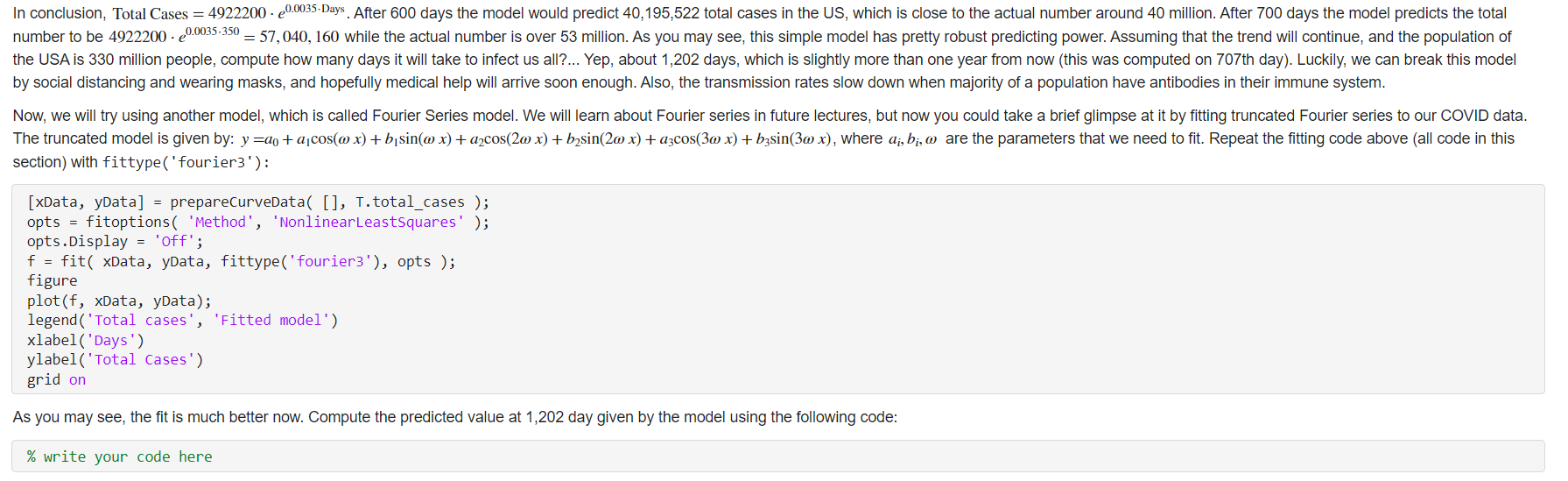
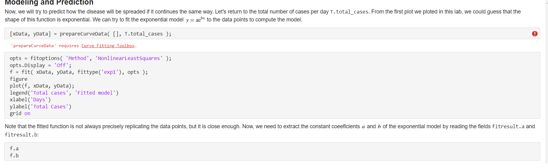
shape of this function is exponential. We can try to fit the exponential model y=aebx to the data points to compute the model. [ xData, yData ]= preparecurveData ([], T.total_cases ); 'prepareCurveData' requires Curve Fitting_Toolbox. opts = fitoptions( 'Method', 'NonlinearLeastSquares'); opts.Display = 'Off'; f = fit( xData, yData, fittype('exp1'), opts ); figure plot(f, xData, yData); legend('Total cases', 'Fitted model') xlabel('Days') ylabel('Total Cases') grid on fitresult.b: f.a f.b In conclusion, Total Cases =4922200ee0.0035-Days. After 600 days the model would predict 40,195,522 total cases in the US, which is close to the actual number around 40 million. After 700 days the model predicts the total number to be 4922200e0.0035350=57,040,160 while the actual number is over 53 million. As you may see, this simple model has pretty robust predicting power. Assuming that the trend will continue, and the population of the USA is 330 million people, compute how many days it will take to infect us all?... Yep, about 1,202 days, which is slightly more than one year from now (this was computed on 707 th day). Luckily, we can break this model by social distancing and wearing masks, and hopefully medical help will arrive soon enough. Also, the transmission rates slow down when majority of a population have antibodies in their immune system. Now, we will try using another model, which is called Fourier Series model. We will learn about Fourier series in future lectures, but now you could take a brief glimpse at it by fitting truncated Fourier series to our COVID data. The truncated model is given by: y=a0+a1cos(x)+b1sin(x)+a2cos(2x)+b2sin(2x)+a3cos(3x)+b3sin(3x), where ai,bi, are the parameters that we need to fit. Repeat the fitting code above (all code in this section) with fittype( ' fourier3' ) : [xData, yData] = preparecurvedata( [], T.total_cases ); opts = fitoptions( 'Method', 'NonlinearLeastSquares' ); opts.Display = 'off'; f = fit( xData, yData, fittype(' fourier3'), opts ); figure plot(f, xData, yData); legend('Total cases', 'Fitted model') xlabel('Days') ylabel(' Total Cases') grid on As you may see, the fit is much better now. Compute the predicted value at 1,202 day given by the model using the following code