Please Use Excel to Complete the Question

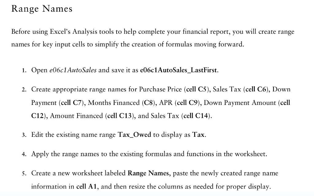
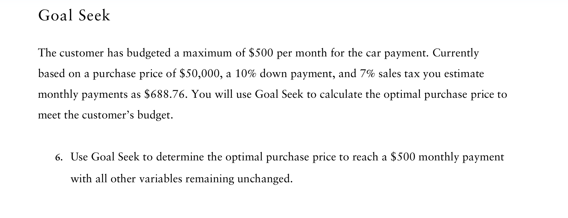
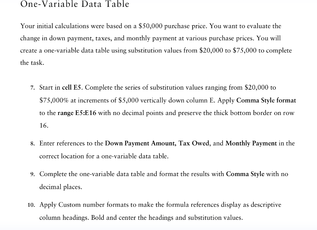
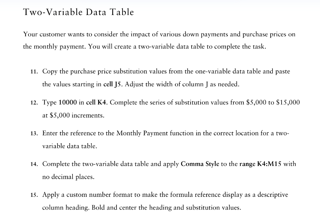
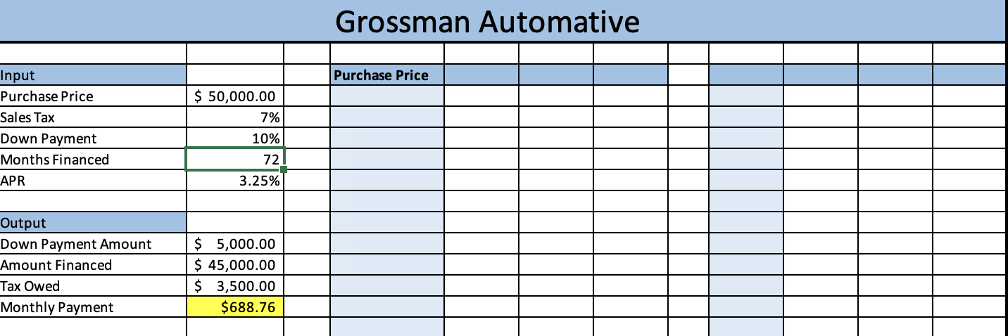
Before using Excel's Analysis tools to help complete your financial report, you will create range names for key input cells to simplify the creation of formulas moving forward. 1. Open e06c1AutoSales and save it as e06c1AutoSales_LastFirst. 2. Create appropriate range names for Purchase Price (cell C5), Sales Tax (cell C6), Down Payment (cell C7), Months Financed (C8), APR (cell C9), Down Payment Amount (cell C12), Amount Financed (cell C13), and Sales Tax (cell C14). 3. Edit the existing name range Tax_Owed to display as Tax. 4. Apply the range names to the existing formulas and functions in the worksheet. 5. Create a new worksheet labeled Range Names, paste the newly created range name information in cell A1, and then resize the columns as needed for proper display. Goal Seek The customer has budgeted a maximum of $500 per month for the car payment. Currently based on a purchase price of $50,000, a 10% down payment, and 7% sales tax you estimate monthly payments as $688.76. You will use Goal Seek to calculate the optimal purchase price to meet the customer's budget. 6. Use Goal Seek to determine the optimal purchase price to reach a $500 monthly payment with all other variables remaining unchanged. Your initial calculations were based on a $50,000 purchase price. You want to evaluate the change in down payment, taxes, and monthly payment at various purchase prices. You will create a one-variable data table using substitution values from $20,000 to $75,000 to complete the task. 7. Start in cell E 5. Complete the series of substitution values ranging from $20,000 to $75,000% at increments of $5,000 vertically down column E. Apply Comma Style format to the range E5:E16 with no decimal points and preserve the thick bottom border on row 16. 8. Enter references to the Down Payment Amount, Tax Owed, and Monthly Payment in the correct location for a one-variable data table. 9. Complete the one-variable data table and format the results with Comma Style with no decimal places. 10. Apply Custom number formats to make the formula references display as descriptive column headings. Bold and center the headings and substitution values. Your customer wants to consider the impact of various down payments and purchase prices on the monthly payment. You will create a two-variable data table to complete the task. 11. Copy the purchase price substitution values from the one-variable data table and paste the values starting in cell J5. Adjust the width of column J as needed. 12. Type 10000 in cell K4. Complete the series of substitution values from $5,000 to $15,000 at $5,000 increments. 13. Enter the reference to the Monthly Payment function in the correct location for a twovariable data table. 14. Complete the two-variable data table and apply Comma Style to the range K4:M15 with no decimal places. 15. Apply a custom number format to make the formula reference display as a descriptive column heading. Bold and center the heading and substitution values. Up to this point, you have created forecasts based on static amounts; however, it is important to plan for several possible finance options. To help you analyze best, worst, and most likely outcomes, you will use Scenario Manager. 16. Create a scenario named Best Case, using Purchase Price and Months Financed. Enter these values for the scenario: 40000 , and 36 . 17. Create a second scenario named Worst Case, using the same changing cells. Enter these values for the scenario: 50000 , and 72 . 18. Create a third scenario named Most Likely, using the same changing cells. Enter these values for the scenario: 45000 , and 60 . 19. Generate a Scenario Summary report based on Monthly Payment. 20. Format the summary as discussed in the chapter. Grossman Automative Before using Excel's Analysis tools to help complete your financial report, you will create range names for key input cells to simplify the creation of formulas moving forward. 1. Open e06c1AutoSales and save it as e06c1AutoSales_LastFirst. 2. Create appropriate range names for Purchase Price (cell C5), Sales Tax (cell C6), Down Payment (cell C7), Months Financed (C8), APR (cell C9), Down Payment Amount (cell C12), Amount Financed (cell C13), and Sales Tax (cell C14). 3. Edit the existing name range Tax_Owed to display as Tax. 4. Apply the range names to the existing formulas and functions in the worksheet. 5. Create a new worksheet labeled Range Names, paste the newly created range name information in cell A1, and then resize the columns as needed for proper display. Goal Seek The customer has budgeted a maximum of $500 per month for the car payment. Currently based on a purchase price of $50,000, a 10% down payment, and 7% sales tax you estimate monthly payments as $688.76. You will use Goal Seek to calculate the optimal purchase price to meet the customer's budget. 6. Use Goal Seek to determine the optimal purchase price to reach a $500 monthly payment with all other variables remaining unchanged. Your initial calculations were based on a $50,000 purchase price. You want to evaluate the change in down payment, taxes, and monthly payment at various purchase prices. You will create a one-variable data table using substitution values from $20,000 to $75,000 to complete the task. 7. Start in cell E 5. Complete the series of substitution values ranging from $20,000 to $75,000% at increments of $5,000 vertically down column E. Apply Comma Style format to the range E5:E16 with no decimal points and preserve the thick bottom border on row 16. 8. Enter references to the Down Payment Amount, Tax Owed, and Monthly Payment in the correct location for a one-variable data table. 9. Complete the one-variable data table and format the results with Comma Style with no decimal places. 10. Apply Custom number formats to make the formula references display as descriptive column headings. Bold and center the headings and substitution values. Your customer wants to consider the impact of various down payments and purchase prices on the monthly payment. You will create a two-variable data table to complete the task. 11. Copy the purchase price substitution values from the one-variable data table and paste the values starting in cell J5. Adjust the width of column J as needed. 12. Type 10000 in cell K4. Complete the series of substitution values from $5,000 to $15,000 at $5,000 increments. 13. Enter the reference to the Monthly Payment function in the correct location for a twovariable data table. 14. Complete the two-variable data table and apply Comma Style to the range K4:M15 with no decimal places. 15. Apply a custom number format to make the formula reference display as a descriptive column heading. Bold and center the heading and substitution values. Up to this point, you have created forecasts based on static amounts; however, it is important to plan for several possible finance options. To help you analyze best, worst, and most likely outcomes, you will use Scenario Manager. 16. Create a scenario named Best Case, using Purchase Price and Months Financed. Enter these values for the scenario: 40000 , and 36 . 17. Create a second scenario named Worst Case, using the same changing cells. Enter these values for the scenario: 50000 , and 72 . 18. Create a third scenario named Most Likely, using the same changing cells. Enter these values for the scenario: 45000 , and 60 . 19. Generate a Scenario Summary report based on Monthly Payment. 20. Format the summary as discussed in the chapter. Grossman Automative