Please use Python.

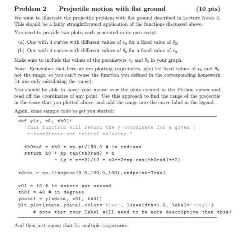
For the following exercises, write your code in one py file for each problem (or part for problem 2). Please, name each script with your name, and the problem number. For example "buerki_hw05-p1.py". You will also need to submit the plots you have created. Use a similar naming scheme for your plot files, for erample 'buerki hw05-p2a-plot.pdf" for the plot created in part b) of problem 2. When submitting in Gradescope, you can either select all files to submit one at a time, or submit one zipped file that contains all your scripts and plots. Make sure that your scripts run without error in order to get credit. Do not hesitate to ask for help if needed! Problem 2 Projectile motion with flat ground (10 pts) We want to illustrate the projectile problem with flat ground described in Lecture Notes 4. This should be a fairly straightforward application of the functions discussed above. You need to provide two plots, each generated in its own script: (a) One with 4 curves with different values of vo for a fixed value of 6o; (b) One with 4 curves with different values of 8, for a fixed value of to. Make sure to include the values of the parameters vo and 8, in your graph. Note: Remember that here we are plotting trajectories, y(r) for fixed values of ve and 8o. not the range, so you can't reuse the function you defined in the corresponding homework (it was only calculating the range). You should be able to hover your mouse over the plots created in the Python viewer and read off the coordinates of any point. Use this approach to find the range of the projectile in the cases that you plotted above, and add the range into the curve label in the legend. Again, some sample code to get you started: def y(x, vo, tho): "This function will return the y-coordinate for a given x-coordinate and initial velocity." thorad = tho + np. pi/180.0 # in radians return ho + np. tan (thorad) + x - (g* ***2)/(2 + v0**2*np.cos(thorad)**2) xdata = np.linspace (0.0,100.0, 1001, endpoint-True) v01 - 10 # in meters per second th01 = 40 # in degrees data1 = y(xdata, voi, th01) plt.plot(xdata, ydata1, color='blue', linewidth=1.0, label='traji') # note that your label will need to be more descriptive than this! And then just repeat that for multiple trajectories