Please write the matlab code as well as send the matlab file to syedfaeque110

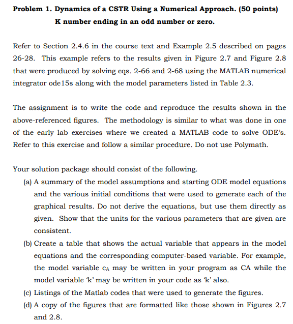
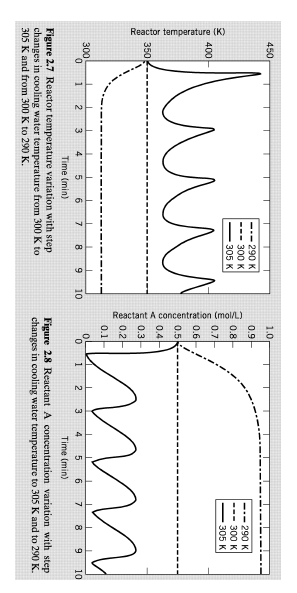
Problem 1. Dynamics of a CSTR Using a Numerical Approach. (50 points) K number ending in an odd number or zero. Refer to Section 2.4.6 in the course text and Example 2.5 described on pages 26-28. This example refers to the results given in Figure 2.7 and Figure 2.8 that were produced by solving eqs. 2-66 and 2-68 using the MATLAB numerical integrator ode 15s along with the model parameters listed in Table 2.3. The assignment is to write the code and reproduce the results shown in the above-referenced figures. The methodology is similar to what was done in one of the early lab exercises where we created a MATLAB code to solve ODE's. Refer to this exercise and follow a similar procedure. Do not use Polymath. Your solution package should consist of the following. (a) A summary of the model assumptions and starting ODE model equations and the various initial conditions that were used to generate each of the graphical results. Do not derive the equations, but use them directly as given. Show that the units for the various parameters that are given are consistent. (b) Create a table that shows the actual variable that appears in the model equations and the corresponding computer-based variable. For example, the model variable cA may be written in your program as CA while the model variable ' k ' may be written in your code as ' k ' also. (c) Listings of the Matlab codes that were used to generate the figures. (d) A copy of the figures that are formatted like those shown in Figures 2.7 and 2.8 . Figure 2.7 Reactor temperature variation with step Figure 2.8 Reactant A concentration variation with step changes in cooling water temperature from 300K to changes in cooling water temperature to 305K and to 290K. 305K and from 300K to 290K. Problem 1. Dynamics of a CSTR Using a Numerical Approach. (50 points) K number ending in an odd number or zero. Refer to Section 2.4.6 in the course text and Example 2.5 described on pages 26-28. This example refers to the results given in Figure 2.7 and Figure 2.8 that were produced by solving eqs. 2-66 and 2-68 using the MATLAB numerical integrator ode 15s along with the model parameters listed in Table 2.3. The assignment is to write the code and reproduce the results shown in the above-referenced figures. The methodology is similar to what was done in one of the early lab exercises where we created a MATLAB code to solve ODE's. Refer to this exercise and follow a similar procedure. Do not use Polymath. Your solution package should consist of the following. (a) A summary of the model assumptions and starting ODE model equations and the various initial conditions that were used to generate each of the graphical results. Do not derive the equations, but use them directly as given. Show that the units for the various parameters that are given are consistent. (b) Create a table that shows the actual variable that appears in the model equations and the corresponding computer-based variable. For example, the model variable cA may be written in your program as CA while the model variable ' k ' may be written in your code as ' k ' also. (c) Listings of the Matlab codes that were used to generate the figures. (d) A copy of the figures that are formatted like those shown in Figures 2.7 and 2.8 . Figure 2.7 Reactor temperature variation with step Figure 2.8 Reactant A concentration variation with step changes in cooling water temperature from 300K to changes in cooling water temperature to 305K and to 290K. 305K and from 300K to 290K