PLZ SOLVE AS MUCH AS POSSIBLE!!

APPENDIX TABLE LINK : https://www.webassign.net/mendstat15/mendstat15_appendix_tables.pdf

Q13B

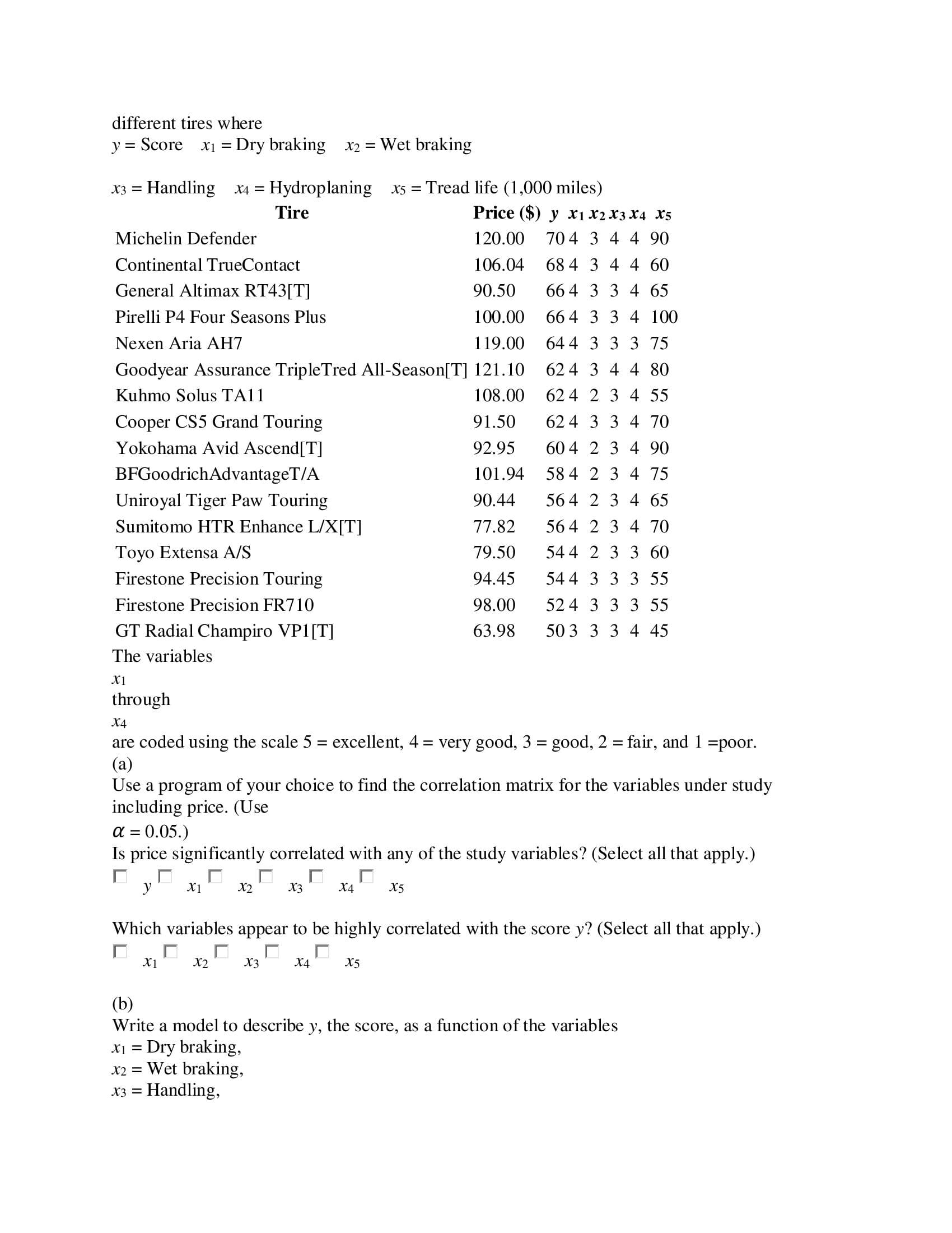
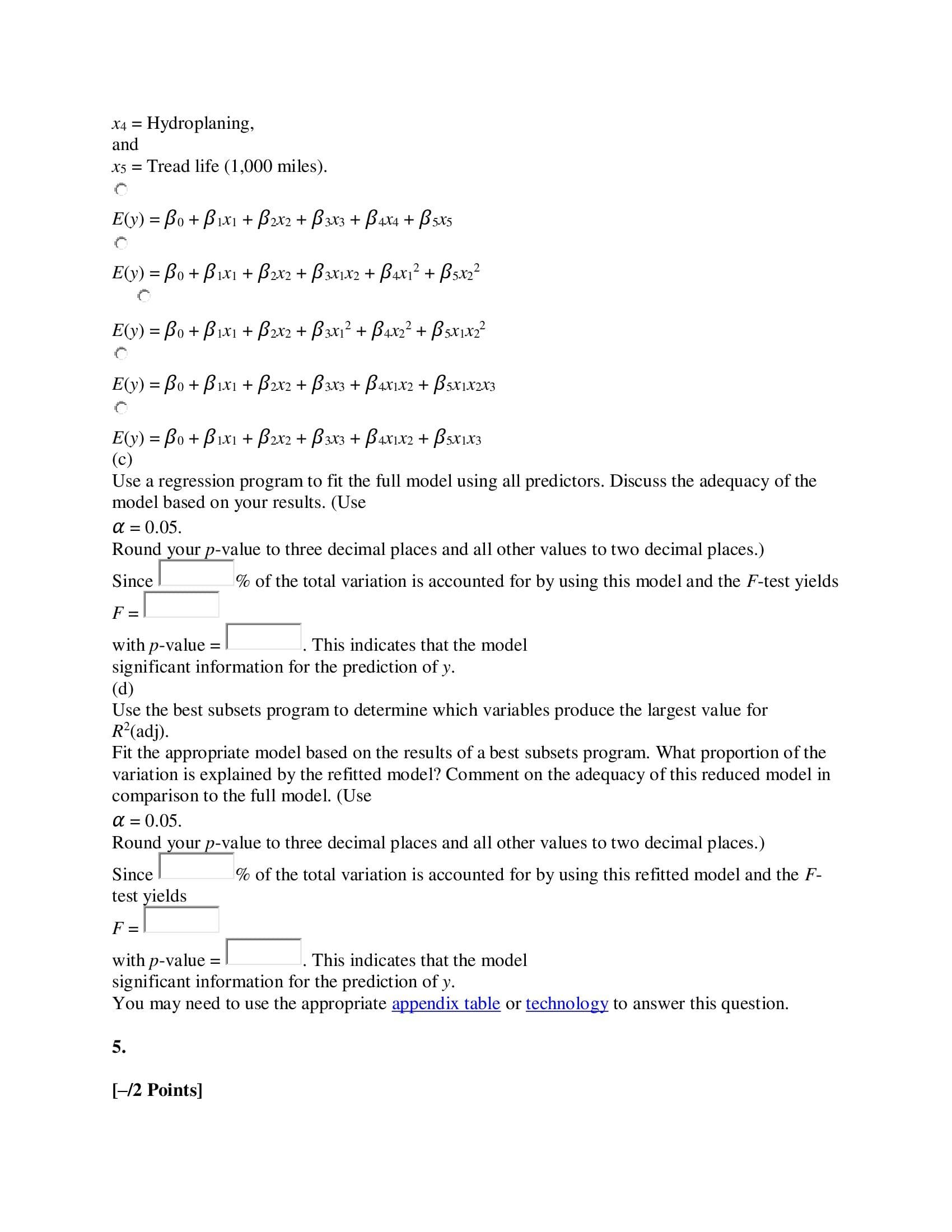
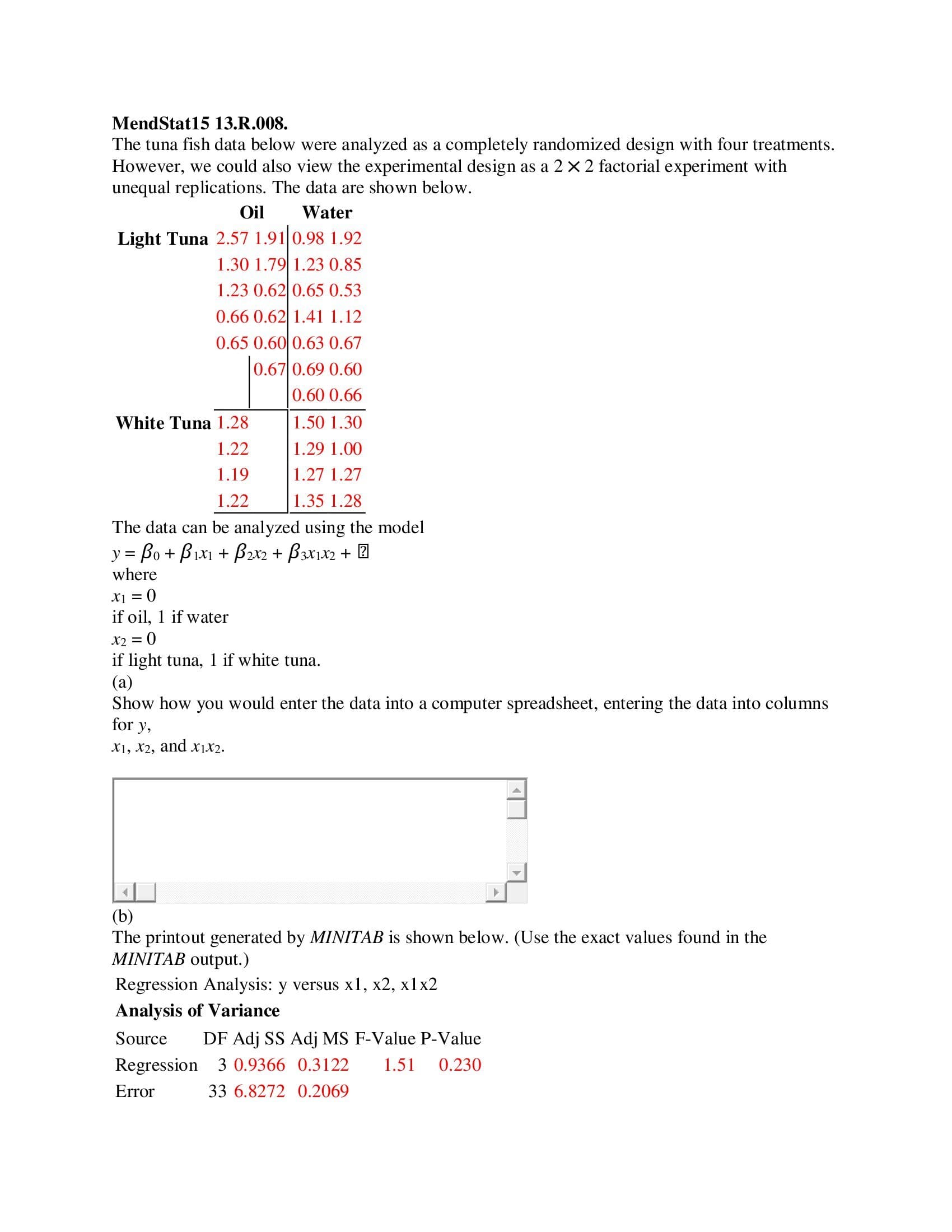
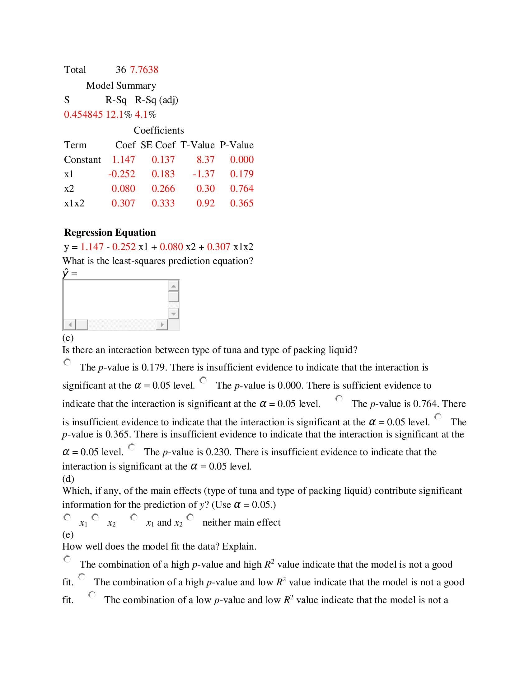
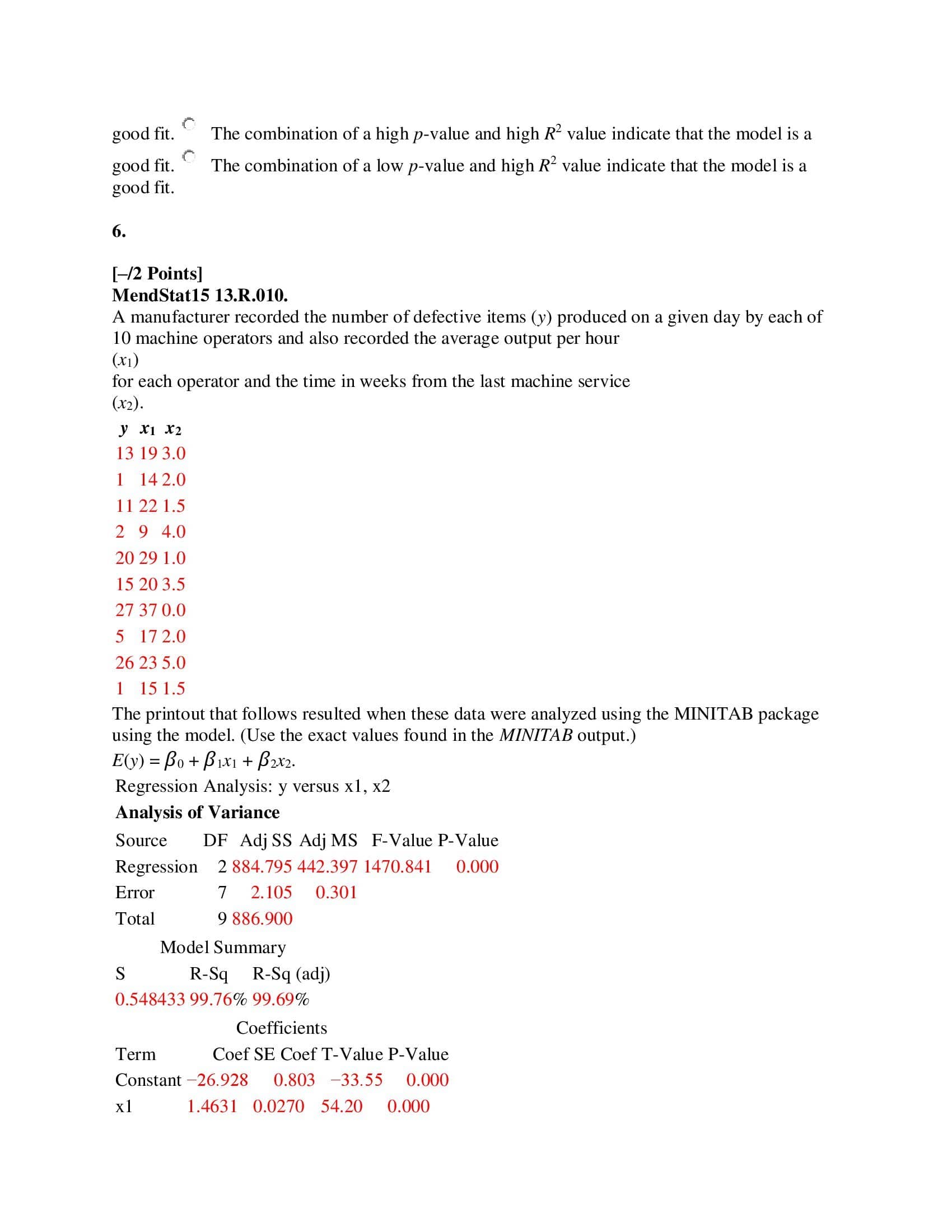
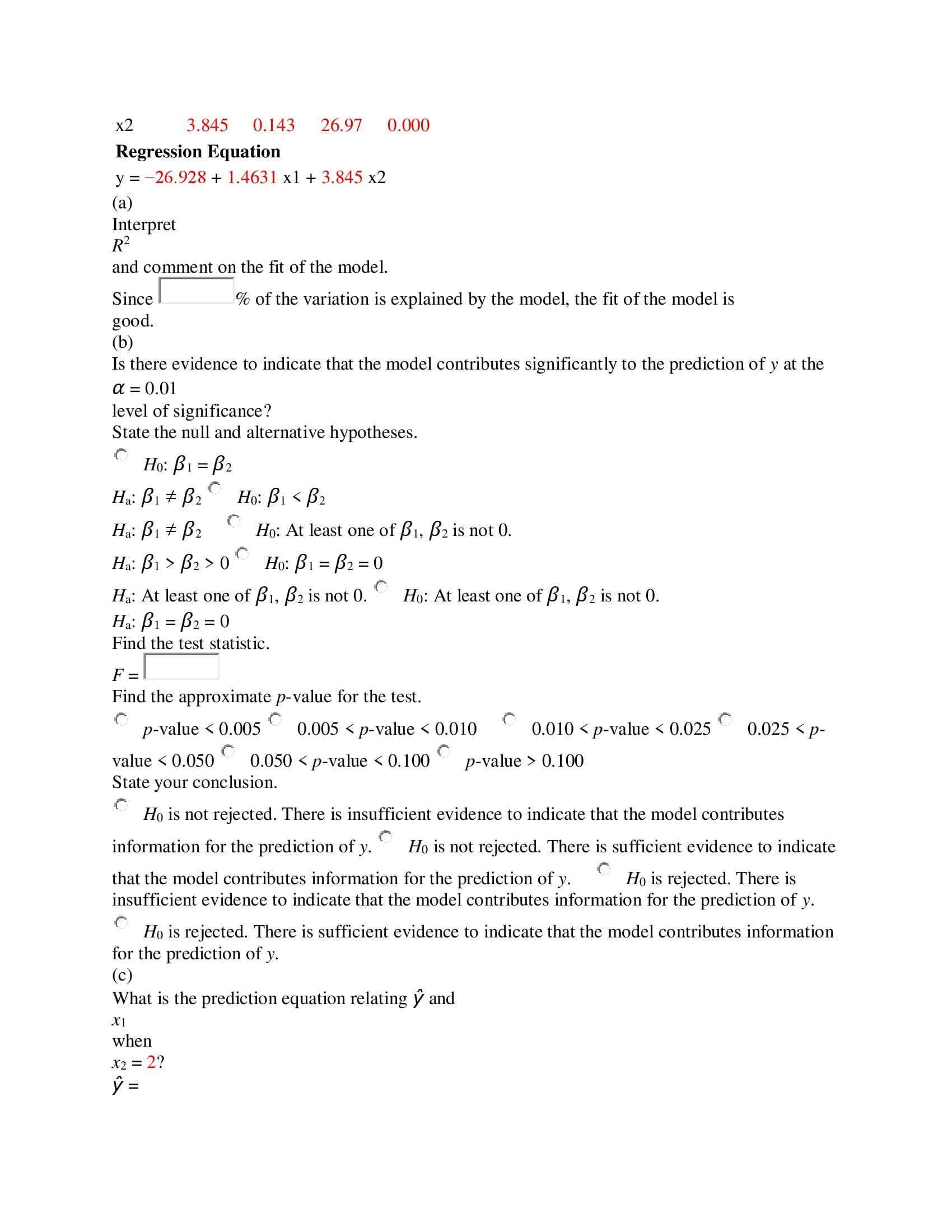
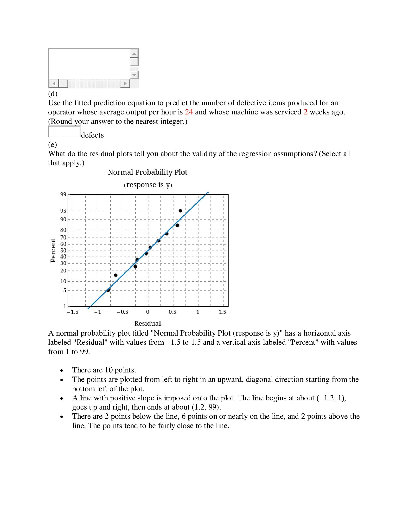
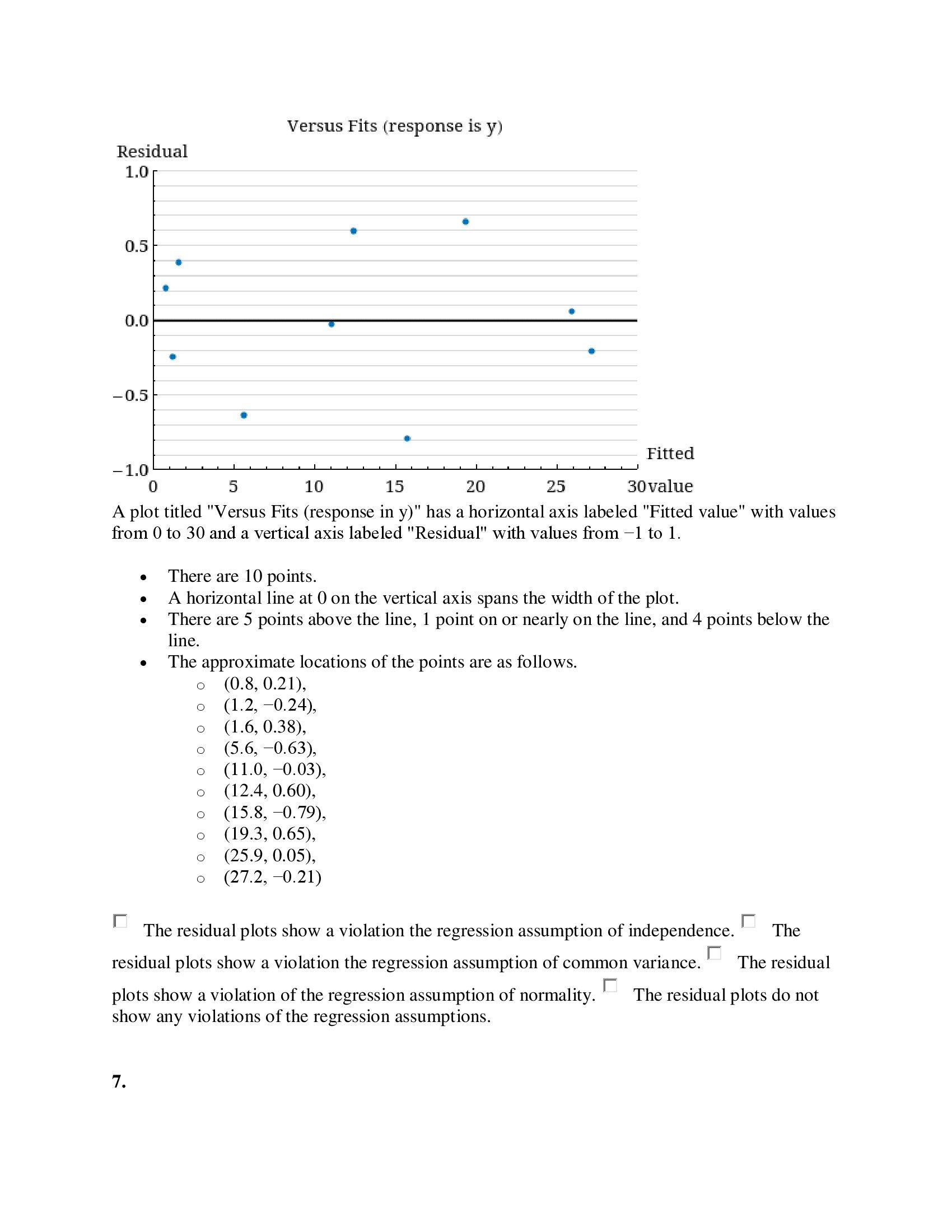
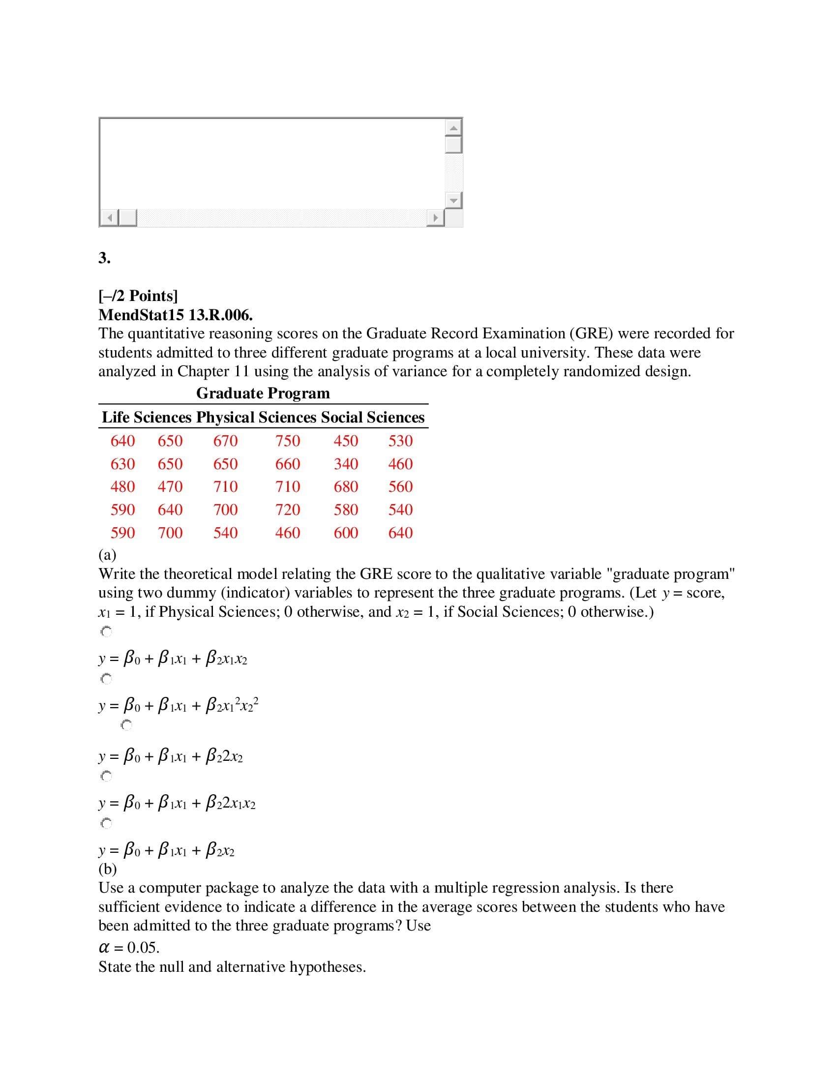
3. [12 Points] MendStatlS 13.R.006. The quantitative reasoning scores on the Graduate Record Examination (GRE) were recorded for students admitted to three different graduate programs at a local university. These data were analyzed in Chapter 11 using the analysis of variance for a completely randomized design. Graduate Program Life Sciences Physical Sciences Social Sciences 640 650 670 750 450 530 630 650 650 660 340 460 480 470 710 710 680 560 590 640 700 720 580 540 590 700 540 460 600 640 (a) Write the theoretical model relating the GRE score to the qualitative variable "graduate program" using two dummy (indicator) variables to represent the three graduate programs. (Let y = score, x1 = 1, if Physical Sciences; 0 otherwise, and x2 = 1, if Social Sciences; 0 otherwise.) (II. y = 30 +31x1+ Bzxrxz r' y = [5'0 + 3m + 'mzxzz It" y = [30 +31X1 + 322162 If\" y = 30 + B1131 + 22x1x2 r. y = o+m + zxz (b) Use a computer package to analyze the data with a multiple regression analysis. Is there sufcient evidence to indicate a difference in the average scores between the students who have been admitted to the three graduate programs? Use a = 0.05. State the null and alternative hypotheses. Ho: At least one of B1, B2 is not 0. Ha: B1 = P2 = 0 Ho: At least one of B1, B2 is not 0. Ha: B1> B2> 0 Ho: BI 0.100 State your conclusion. Ho is not rejected. There is sufficient evidence to indicate there is a difference in the average scores between the students who have been admitted to the three graduate programs. Ho is rejected. There is insufficient evidence to indicate there is a difference in the average scores between the students who have been admitted to the three graduate programs. Ho is rejected. There is sufficient evidence to indicate there is a difference in the average scores between the students who have been admitted to the three graduate programs. Ho is not rejected. There is insufficient evidence to indicate there is a difference in the average scores between the students who have been admitted to the three graduate programs. C Comment on the fit of the model and any regression assumptions that may have been violated. Summarize your results in a report, including printouts and graphs if possible. You may need to use the appropriate appendix table or technology to answer this question. 4. [-/2 Points] MendStat15 13.R.007. Performance tires used to be fitted mostly on sporty or luxury vehicles. Now they come standard on many standard vehicles. The data that follow are abstracted from a report on all-season tires by Consumer Reports/ in which several aspects of performance were evaluated for n = 16different tires where y = Score x1 = Dry braking x2 = Wet braking x3 = Handling x4 = Hydroplaning x5 = Tread life (1,000 miles) Tire Price ($) y x1X2X3X4 X5 Michelin Defender 120.00 70 4 3 4 4 90 Continental TrueContact 106.04 68 4 3 4 4 60 General Altimax RT43[T] 90.50 664 3 3 4 65 Pirelli P4 Four Seasons Plus 100.00 66 4 3 3 4 100 Nexen Aria AH7 119.00 64 4 3 3 3 75 Goodyear Assurance Triple Tred All-Season[T] 121.10 624 3 4 4 80 Kuhmo Solus TAll 108.00 62 4 2 3 4 55 Cooper CS5 Grand Touring 91.50 62 4 3 3 4 70 Yokohama Avid Ascend[T] 92.95 60 4 2 3 4 90 BFGoodrich AdvantageT/A 101.94 584 2 3 4 75 Uniroyal Tiger Paw Touring 90.44 564 2 3 4 65 Sumitomo HTR Enhance L/X[T] 77.82 56 4 2 3 4 70 Toyo Extensa A/S 79.50 54 4 2 3 3 60 Firestone Precision Touring 94.45 54 4 3 3 3 55 Firestone Precision FR710 98.00 52 4 3 3 3 55 GT Radial Champiro VPI [T] 63.98 503 3 3 4 45 The variables X1 through X4 are coded using the scale 5 = excellent, 4 = very good, 3 = good, 2 = fair, and 1 =poor. (a) Use a program of your choice to find the correlation matrix for the variables under study including price. (Use a = 0.05.) Is price significantly correlated with any of the study variables? (Select all that apply.) y x x2 x3 X4 x Which variables appear to be highly correlated with the score y? (Select all that apply.) X1 X2 X3 x4 X5 (b) Write a model to describe y, the score, as a function of the variables x1 = Dry braking, x2 = Wet braking, x3 = Handling,x4 = Hydroplaning, and x5 = Tread life (1,000 miles). I!\" E(y) =30 +1x1+2x2 + 53x3 +b'm +[J'sxs r' E(y) = 30 + 31x1 + 3m + SXlxz + 34x12 + 35x22 1* EO') = 30 + 3m + 32262 + 33x12 + 34ch2 + sxlxzz r. E(y) = g + 1x1+ zxz + 33m + [34.36110 + sxlxzxs (I. E0') = 30 + IXI + 32x2 + 53x3 + ulxz + shxs (C) Use a regression program to t the full model using all predictors. Discuss the adequacy of the model based on your results. (Use a = 0.05. Round your g-value to three decimal places and all other values to two decimal places.) Since F = I with p-value = I . This indicates that the model signicant information for the prediction of y. (d) Use the best subsets program to detcmline which variables produce the largest value for R2(adj). Fit the appropriate model based on the results of a best subsets program. What proportion of the variation is explained by the retted model? Comment on the adequacy of this reduced model in comparison to the full model. (Use a = 0.05. Round your g-value to three decimal places and all other values to two decimal places.) % of the total variatiOn is accounted for by using this model and the F -test yields Since test ields F = i withp-value = I . This indicates that the model signicant information for the prediction of y. You may need to use the appropriate appendix table or technology to answer this question. % of the total variation is accounted for by using this retted model and the F- 5' [12 Points] MendStatlS 13.R.008. The tuna sh data below were analyzed as a completely randomized design with four treatments. However, we could also view the experimental design as a 2 x 2 factorial experiment with unequal replications. The data are shown below. Oil Water Light Tuna 2.57 1.91 0.98 1.92 1,301.79 1.23 0.85 1.23 0.62 0.65 0.53 0.66 0.62 1.41 1.12 0.65 0.60 0.63 0.67 0.67 0.69 0.60 0.60 0.66 White Tuna 1.28 1.50 1.30 1.22 1.29 1.00 1.19 1.27 1.27 1.22 1.35 1.28 The data can be analyzed using the model y=o+lx1+2x2+3x1x2+ where .761 = 0 if oil, 1 if water X2 = 0 if light tuna, 1 if white tuna. (a) Show how you would enter the data into a computer spreadsheet, entering the data into columns for y, x1, x2, and x1362. _..l' (b) The printout generated by MINITAB is shown below. (Use the exact values found in the MINI TAB output.) Regression Analysis: y versus x1, x2, x1 x2 Analysis of Variance Source DF Adj SS Adj MS F-Value P-Value Regression 3 0.9366 0.3122 1.51 0.230 Error 33 6.8272 0.2069 Total 36 7.7638 Model Summary S R-Sq R-Sq (adj) 0.454845 12.1% 4.1% Coefficients Term Coef SE Coef T-Value P-Value Constant 1.147 0.137 8.37 0.000 -0.252 0.183 1.37 0.179 X2 0.080 0.266 0.30 0.764 x1x2 0.307 0.333 0.92 0.365 Regression Equation y = 1.147 - 0.252 x1 + 0.080 x2 + 0.307 x1x2 What is the least-squares prediction equation? y = (c) Is there an interaction between type of tuna and type of packing liquid? The p-value is 0.179. There is insufficient evidence to indicate that the interaction is significant at the a = 0.05 level. The p-value is 0.000. There is sufficient evidence to indicate that the interaction is significant at the a = 0.05 level. The p-value is 0.764. There is insufficient evidence to indicate that the interaction is significant at the a = 0.05 level. The p-value is 0.365. There is insufficient evidence to indicate that the interaction is significant at the a = 0.05 level. The p-value is 0.230. There is insufficient evidence to indicate that the interaction is significant at the a = 0.05 level. (d) Which, if any, of the main effects (type of tuna and type of packing liquid) contribute significant information for the prediction of y? (Use a = 0.05.) C X1 * 2 x1 and x2 neither main effect (e) How well does the model fit the data? Explain. The combination of a high p-value and high R value indicate that the model is not a good fit. The combination of a high p-value and low R value indicate that the model is not a good fit. The combination of a low p-value and low R2 value indicate that the model is not agood fit. The combination of a high p-value and high R' value indicate that the model is a good fit. The combination of a low p-value and high R value indicate that the model is a good fit. 6. [-/2 Points] MendStat15 13.R.010. A manufacturer recorded the number of defective items (y) produced on a given day by each of 10 machine operators and also recorded the average output per hour (x1) for each operator and the time in weeks from the last machine service (x2). y x1 X2 13 19 3.0 1 14 2.0 1 1 22 1.5 2 9 4.0 20 29 1.0 15 20 3.5 27 37 0.0 5 172.0 26 23 5.0 1 15 1.5 The printout that follows resulted when these data were analyzed using the MINITAB package using the model. (Use the exact values found in the MINITAB output.) E(y) = Bo + PIXI + B2x2. Regression Analysis: y versus x1, x2 Analysis of Variance Source DF Adj SS Adj MS F-Value P-Value Regression 2 884.795 442.397 1470.841 0.000 Error 7 2.105 0.301 Total 9 886.900 Model Summary S R-Sq R-Sq (adj) 0.548433 99.76% 99.69% Coefficients Term Coef SE Coef T-Value P-Value Constant -26.928 0.803 -33.55 0.000 x1 1.4631 0.0270 54.20 0.000x2 3.845 0.143 26.97 0.000 Regression Equation y = -26.928 + 1.4631 x1 + 3.845 x2 (a) Interpret R2 and comment on the fit of the model. Since of the variation is explained by the model, the fit of the model is good. (b Is there evidence to indicate that the model contributes significantly to the prediction of y at the a = 0.01 level of significance? State the null and alternative hypotheses. C Ho: B1 = B2 Ha: B1 # B2 Ho: B1 B2> O Ho: B1 = B2 = 0 Ha: At least one of B1, B2 is not O. Ho: At least one of B1, B2 is not 0. Ha: B1 = B2 = 0 Find the test statistic. F = Find the approximate p-value for the test. p-value 0.100 State your conclusion. C Ho is not rejected. There is insufficient evidence to indicate that the model contributes information for the prediction of y. Ho is not rejected. There is sufficient evidence to indicate that the model contributes information for the prediction of y. Ho is rejected. There is insufficient evidence to indicate that the model contributes information for the prediction of y. Ho is rejected. There is sufficient evidence to indicate that the model contributes information for the prediction of y. (c) What is the prediction equation relating y and X1 when X2 = 2? y =(d Use the fitted prediction equation to predict the number of defective items produced for an operator whose average output per hour is 24 and whose machine was serviced 2 weeks ago. Round your answer to the nearest integer.) defects (e) What do the residual plots tell you about the validity of the regression assumptions? (Select all that apply.) Normal Probability Plot (response is y) 99 95 Percent -1.5 -0.5 0 0.5 1.5 Residual A normal probability plot titled "Normal Probability Plot (response is y)" has a horizontal axis labeled "Residual" with values from -1.5 to 1.5 and a vertical axis labeled "Percent" with values from 1 to 99. There are 10 points. . The points are plotted from left to right in an upward, diagonal direction starting from the bottom left of the plot A line with positive slope is imposed onto the plot. The line begins at about (-1.2, 1), goes up and right, then ends at about (1.2, 99). There are 2 points below the line, 6 points on or nearly on the line, and 2 points above the line. The points tend to be fairly close to the line.Versus Fits (reap unse is 3!] Residual 1.0 {1.0 {'.|.5 Fitted 1.1) {J 5 10 15 2D 25 Svalue A plot titled "Versus Fits (response in y)" has a horizontal axis labeled "Fitted value" with values from 0 to 30 and a vertical axis labeled "Residual" with values from 1 to l. . There are 10 points. . A horizontal line at 0 on the vertical axis spans the width of the plot. . There are 5 points above the line, 1 point on or nearly on the line, and 4 points below the line. . The approximate locations of the points are as follows. (0.8, 0.21), (1.2, 70.24), (1.6, 0.38), (5.6, 70.63), (11.0, 70.03), (12.4, 0.60), (15.8, 0.79), (19.3, 0.65), (25.9, 0.05), (27.2, 70.21) OOOOOOOOOO I l The residual plots show a violation the regression assumption of independence. The I residual plots show a violation the regression assumption of common variance. The residual plots show a violation of the regression assumption of normality. ' show any violations of the regression assumptions. The residual plots do not