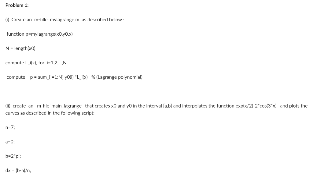
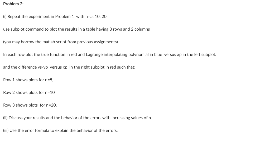
Problem 1: (i). Create an m-fille mylagrange.m as described below: function p=mylagrange(x0,70,x) N = length(x0) compute L_i(x), for i=1,2,...,N compute p = sum_{i=1:N} yo(i) "L_i(x) % (Lagrange polynomial) (ii) create an m-file 'main_lagrange' that creates XO and yo in the interval (a,b) and interpolates the function exp(x/2)-2*cos(3*x) and plots the curves as described in the following script: n=7; a=0; b=2*pi; dx = (b-a); XO=0:dx:b; f=@(x) exp(x/2)-2* cos(3*x); yO=f(x0); np=100; dxp=(b-a)p; xp=a:dxp:b; ys=f(xp); yp=mylagrange(x0,70,xp); plot(xp,yp); hold on plot(xp.ys) plot(x0,70,*) (iii) Print your results. (iv) Are your results correct? Explain why or why not? Problem 2: (i) Repeat the experiment in Problem 1 with n=5, 10, 20 use subplot command to plot the results in a table having 3 rows and 2 columns (you may borrow the matlab script from previous assignments) In each row plot the true function in red and Lagrange interpolating polynomial in blue versus xp in the left subplot. and the difference ys-yp versus xp in the right subplot in red such that: Row 1 shows plots for n=5, Row 2 shows plots for n=10 Row 3 shows plots for n=20. (ii) Discuss your results and the behavior of the errors with increasing values of n. (iii) Use the error formula to explain the behavior of the errors. Problem 1: (i). Create an m-fille mylagrange.m as described below: function p=mylagrange(x0,70,x) N = length(x0) compute L_i(x), for i=1,2,...,N compute p = sum_{i=1:N} yo(i) "L_i(x) % (Lagrange polynomial) (ii) create an m-file 'main_lagrange' that creates XO and yo in the interval (a,b) and interpolates the function exp(x/2)-2*cos(3*x) and plots the curves as described in the following script: n=7; a=0; b=2*pi; dx = (b-a); XO=0:dx:b; f=@(x) exp(x/2)-2* cos(3*x); yO=f(x0); np=100; dxp=(b-a)p; xp=a:dxp:b; ys=f(xp); yp=mylagrange(x0,70,xp); plot(xp,yp); hold on plot(xp.ys) plot(x0,70,*) (iii) Print your results. (iv) Are your results correct? Explain why or why not? Problem 2: (i) Repeat the experiment in Problem 1 with n=5, 10, 20 use subplot command to plot the results in a table having 3 rows and 2 columns (you may borrow the matlab script from previous assignments) In each row plot the true function in red and Lagrange interpolating polynomial in blue versus xp in the left subplot. and the difference ys-yp versus xp in the right subplot in red such that: Row 1 shows plots for n=5, Row 2 shows plots for n=10 Row 3 shows plots for n=20. (ii) Discuss your results and the behavior of the errors with increasing values of n. (iii) Use the error formula to explain the behavior of the errors