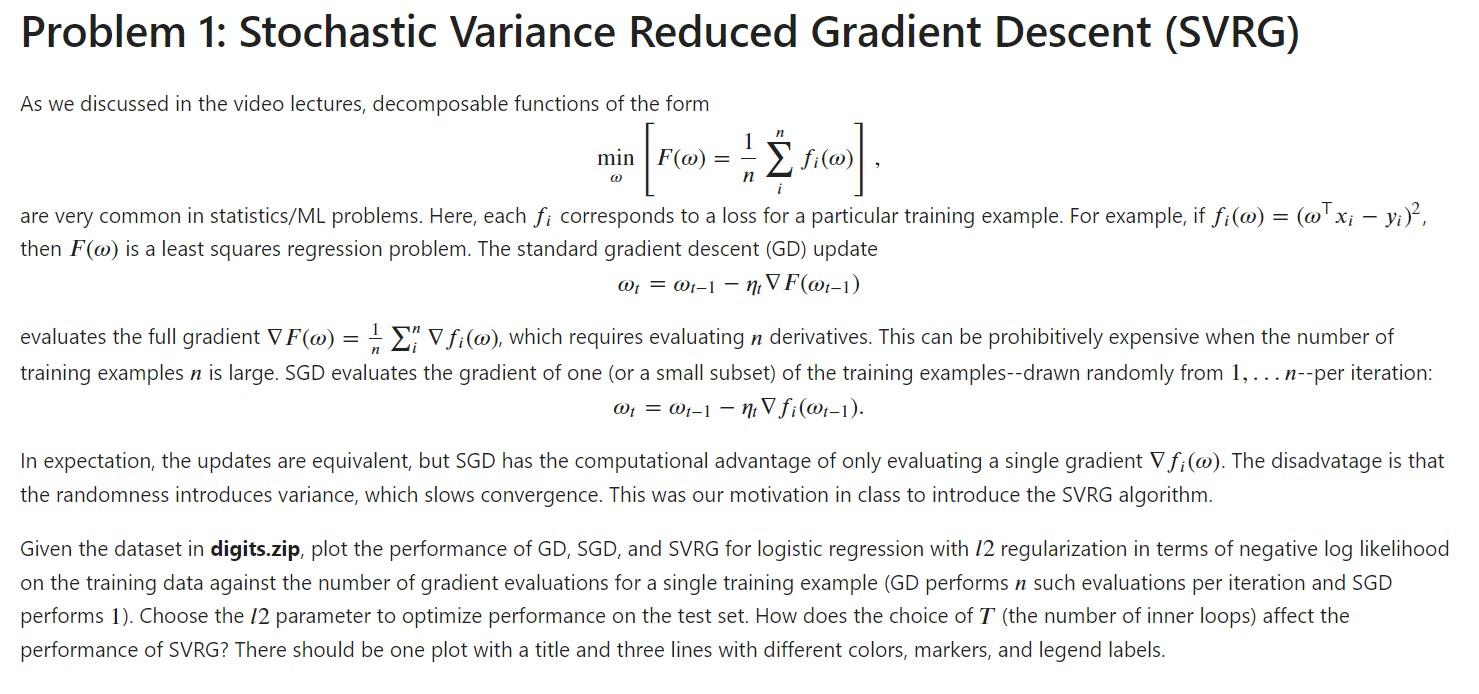
Question: # Problem 1: Stochastic Variance Reduced Gradient Descent (SVRG) As we discussed in the video lectures, decomposable functions of the form $$ min_{omega} left [

# Problem 1: Stochastic Variance Reduced Gradient Descent (SVRG)
As we discussed in the video lectures, decomposable functions of the form $$ \min_{\omega} \left [ F(\omega) = \frac{1}{n} \sum_i^n f_i(\omega) ight ], $$ are very common in statistics/ML problems. Here, each $f_i$ corresponds to a loss for a particular training example. For example, if $f_i(\omega) = (\omega^\top x_i - y_i)^2$, then $F(\omega)$ is a least squares regression problem. The standard gradient descent (GD) update $$ \omega_t = \omega_{t-1} - \eta_t abla F(\omega_{t-1}) $$
evaluates the full gradient $ abla F(\omega) = \frac{1}{n} \sum_i^n abla f_i(\omega)$, which requires evaluating $n$ derivatives. This can be prohibitively expensive when the number of training examples $n$ is large. SGD evaluates the gradient of one (or a small subset) of the training examples--drawn randomly from ${1,...n}$--per iteration: $$ \omega_t = \omega_{t-1} - \eta_t abla f_i(\omega_{t-1}). $$
In expectation, the updates are equivalent, but SGD has the computational advantage of only evaluating a single gradient $ abla f_i(\omega)$. The disadvatage is that the randomness introduces variance, which slows convergence. This was our motivation in class to introduce the SVRG algorithm.
Given the dataset in **digits.zip**, plot the performance of GD, SGD, and SVRG for logistic regression with $l2$ regularization in terms of negative log likelihood on the training data against the number of gradient evaluations for a single training example (GD performs $n$ such evaluations per iteration and SGD performs $1$). Choose the $l2$ parameter to optimize performance on the test set. How does the choice of $T$ (the number of inner loops) affect the performance of SVRG? There should be one plot with a title and three lines with different colors, markers, and legend labels.
Problem 1: Stochastic Variance Reduced Gradient Descent (SVRG) As we discussed in the video lectures, decomposable functions of the form min[F()=n1infi()], are very common in statistics/ML problems. Here, each fi corresponds to a loss for a particular training example. For example, if fi()=(xiyi)2, then F() is a least squares regression problem. The standard gradient descent (GD) update t=t1tF(t1) evaluates the full gradient F()=n1infi(), which requires evaluating n derivatives. This can be prohibitively expensive when the number of training examples n is large. SGD evaluates the gradient of one (or a small subset) of the training examples--drawn randomly from 1,n--per iteration: t=t1tfi(t1). In expectation, the updates are equivalent, but SGD has the computational advantage of only evaluating a single gradient fi(). The disadvatage is that the randomness introduces variance, which slows convergence. This was our motivation in class to introduce the SVRG algorithm. Given the dataset in digits.zip, plot the performance of GD, SGD, and SVRG for logistic regression with 12 regularization in terms of negative log likelihood on the training data against the number of gradient evaluations for a single training example (GD performs n such evaluations per iteration and SGD performs 1). Choose the l2 parameter to optimize performance on the test set. How does the choice of T (the number of inner loops) affect the performance of SVRG? There should be one plot with a title and three lines with different colors, markers, and legend labels
Step by Step Solution
There are 3 Steps involved in it

Get step-by-step solutions from verified subject matter experts


