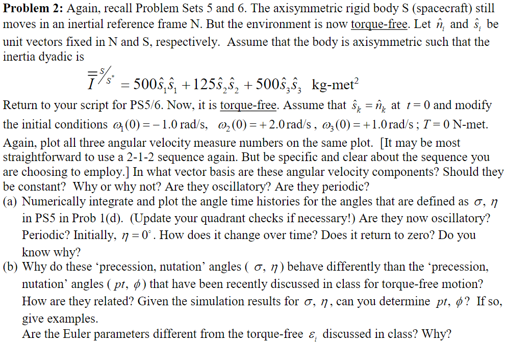
Problem 2: Again, recall Problem Sets 5 and 6. The axisymmetric rigid body S (spacecraft) still moves in an inertial reference frame N. But the environment is now torque-free. Let , and , be unit vectors fixed in N and S, respectively. Assume that the body is axisymmetric such that the inertia dyadic is = - 500 +125 +500 kg-met Return to your script for PS5/6. Now, it is torque-free. Assume that S = n at t=0 and modify the initial conditions (0) = -1.0 rad/s, 2(0) = +2.0 rad/s, @3(0) = +1.0 rad/s; T=0 N-met. Again, plot all three angular velocity measure numbers on the same plot. [It may be most straightforward to use a 2-1-2 sequence again. But be specific and clear about the sequence you are choosing to employ.] In what vector basis are these angular velocity components? Should they be constant? Why or why not? Are they oscillatory? Are they periodic? (a) Numerically integrate and plot the angle time histories for the angles that are defined as , n in PS5 in Prob 1(d). (Update your quadrant checks if necessary!) Are they now oscillatory? Periodic? Initially, n =0. How does it change over time? Does it return to zero? Do you know why? (b) Why do these 'precession, nutation' angles (, 17) behave differently than the 'precession, nutation' angles (pt, 6) that have been recently discussed in class for torque-free motion? How are they related? Given the simulation results for , 1, can you determine pt, ? If so, give examples. Are the Euler parameters different from the torque-free , discussed in class? Why?