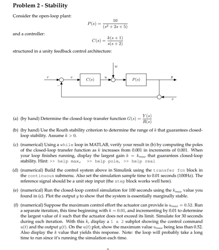
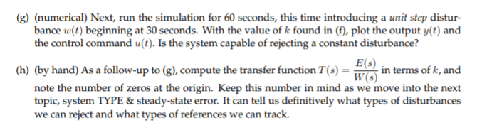
Problem 2 - Stability Consider the open-loop plant: 10 P(s) (32 +2s +5) and a controller: C($) k(s+1) s(s+2) structured in a unity feedback control architecture: u C(s) P(s) Y(8) (a) (by hand) Determine the closed-loop transfer function G(8) = R(S) (b) (by hand) Use the Routh stability criterion to determine the range of k that guarantees closed- loop stability. Assume k > 0. (e) (numerical) Using a while loop in MATLAB, verify your result in (b) by computing the poles of the closed-loop transfer function as k increases from 0.001 in increments of 0.001. When your loop finishes running, display the largest gain k = kmaz that guarantees closed-loop stability. Hint: >> help max, >> help pole, >> help real (d) (numerical) Build the control system above in Simulink using the transfer fcn block in the continuous submenu. Also set the simulation sample time to 0.01 seconds (100Hz). The reference signal should be a unit step input (the step block works well here). (e) (numerical) Run the closed-loop control simulation for 100 seconds using the kmaz value you found in (c). Plot the output y to show that the system is essentially marginally stable. (1) (numerical) Suppose the maximum control effort the actuator can provide is Umar = 0.52. Run a separate iteration, this time beginning with k = 0.01, and incrementing by 0.01 to determine the largest value of k such that the actuator does not exceed its limit. Simulate for 30 seconds during each iteration. With this k, display a 1 x 2 subplot showing the control command u(t) and the output y(t). On the u(t) plot, show the maximum value umaz being less than 0.52. Also display the k value that yields this response. Note: the loop will probably take a long time to run since it's running the simulation each time. (g) (numerical) Next, run the simulation for 60 seconds, this time introducing a unit step distur- bance w(t) beginning at 30 seconds. With the value of k found in (f), plot the output y(t) and the control command u(t). Is the system capable of rejecting a constant disturbance? (h) (by hand) As a follow-up to (g), compute the transfer function T(s) = W(8) note the number of zeros at the origin. Keep this number in mind as we move into the next topic, system TYPE & steady-state error. It can tell us definitively what types of disturbances we can reject and what types of references we can track. E(s) in terms of k, and Problem 2 Include your hand calculations from (a), (b), (h) Include all of your well-commented MATLAB code / Simulink diagrams Include all plots / numerical results from (c)-(g) and answer any of the questions outlined in the problem statements. Provide a brief discussion summarizing your results