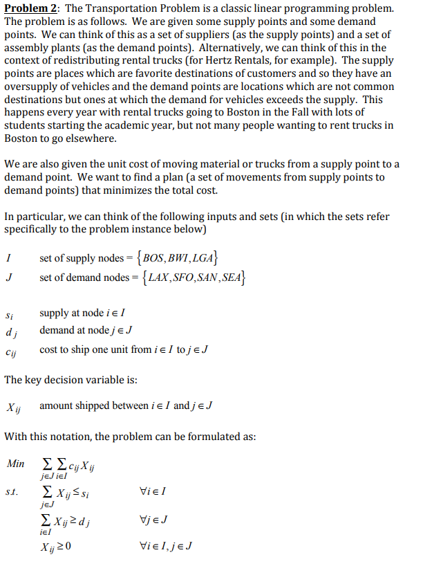
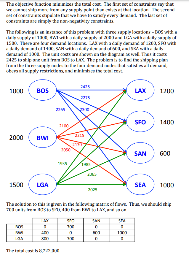
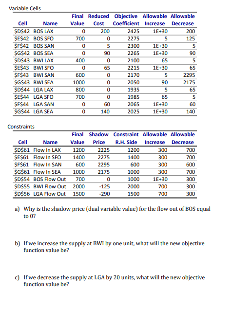
Problem 2: The Transportation Problem is a classic linear programming problem. The problem is as follows. We are given some supply points and some demand points. We can think of this as a set of suppliers (as the supply points) and a set of assembly plants (as the demand points). Alternatively, we can think of this in the context of redistributing rental trucks (for Hertz Rentals, for example). The supply points are places which are favorite destinations of customers and so they have an oversupply of vehicles and the demand points are locations which are not common destinations but ones at which the demand for vehicles exceeds the supply. This happens every year with rental trucks going to Boston in the Fall with lots of students starting the academic year, but not many people wanting to rent trucks in Boston to go elsewhere. We are also given the unit cost of moving material or trucks from a supply point to a demand point. We want to find a plan (a set of movements from supply points to demand points) that minimizes the total cost. In particular, we can think of the following inputs and sets (in which the sets refer specifically to the problem instance below) 1 set of supply nodes = {BOS, BWI,LGA} J set of demand nodes = {LAX, SFO,SAN, SEA} Si dj supply at node i el demand at node je J cost to ship one unit from i el toje J Cij The key decision variable is: amount shipped between i e l and je J With this notation, the problem can be formulated as: Min cy X St. Viel jeJ iel Xij si jeJ Xij? dj Vje J iel X120 Viel, je The objective function minimizes the total cost. The first set of constraints say that we cannot ship more from any supply point than exists at that location. The second set of constraints stipulate that we have to satisfy every demand. The last set of constraints are simply the non-negativity constraints. The following is an instance of this problem with three supply locations - BOS with a daily supply of 1000, BWI with a daily supply of 2000 and LGA with a daily supply of 1500. There are four demand locations: LAX with a daily demand of 1200, SFO with a daily demand of 1400, SAN with a daily demand of 600, and SEA with a daily demand of 1000. The unit costs are shown on the diagram as well. Thus it costs 2425 to ship one unit from BOS to LAX. The problem is to find the shipping plan from the three supply nodes to the four demand nodes that satisfies all demand, obeys all supply restrictions, and minimizes the total cost. 2425 1000 BOS LAX 1200 2275 2265 300 SFO 1400 2100 2000 BWI 2215 2170 2050 SAN 600 1935 1985 2065 1500 LGA SEA 1000 2025 The solution to this is given in the following matrix of flows. Thus, we should ship 700 units from BOS to SFO, 400 from BWI to LAX, and so on. BOS BWI LGA LAX 0 400 800 SFO 700 0 700 SAN 0 600 0 SEA 0 1000 0 The total cost is 8,722,000. Variable Cells Cell Name $D$42 BOS LAX $E$42 BOS SFO $F$42 BOS SAN $G$42 BOS SEA $D$43 BWI LAX $E$43 BWI SFO $F$43 BWI SAN $G$43 BWI SEA $D$44 LGA LAX $E$44 LGA SFO $F$44 LGA SAN $G$44 LGA SEA Final Reduced Objective Allowable Allowable Value Cost Coefficient Increase Decrease 0 200 2425 1E+30 200 700 0 2275 5 125 0 5 2300 1E+30 5 0 90 2265 1E+30 90 400 0 2100 65 5 0 65 2215 1E+30 65 600 0 2170 5 2295 1000 0 2050 90 2175 800 0 1935 5 65 700 0 1985 65 5 0 60 2065 1E+30 60 0 140 2025 1E+30 140 Constraints Final Shadow Constraint Allowable Allowable Cell Name Value Price R.H. Side Increase Decrease $D$61 Flow In LAX 1200 2225 1200 300 700 $E$61 Flow In SFO 1400 2275 1400 300 700 $F$61 Flow In SAN 600 2295 600 300 600 $G$61 Flow In SEA 1000 2175 1000 300 700 $D$54 BOS Flow Out 700 0 1000 1E+30 300 $D$55 BWI Flow Out 2000 -125 2000 700 300 $D$56 LGA Flow Out 1500 -290 1500 700 300 a) Why is the shadow price (dual variable value) for the flow out of BOS equal to 02 b) If we increase the supply at BWI by one unit, what will the new objective function value be? c) If we decrease the supply at LGA by 20 units, what will the new objective function value be? d) If the demand at SAN increases by 5 units, what will the new objective function value be? e) If the demand at SFO decreases by 10 units, what will the new objective function value be