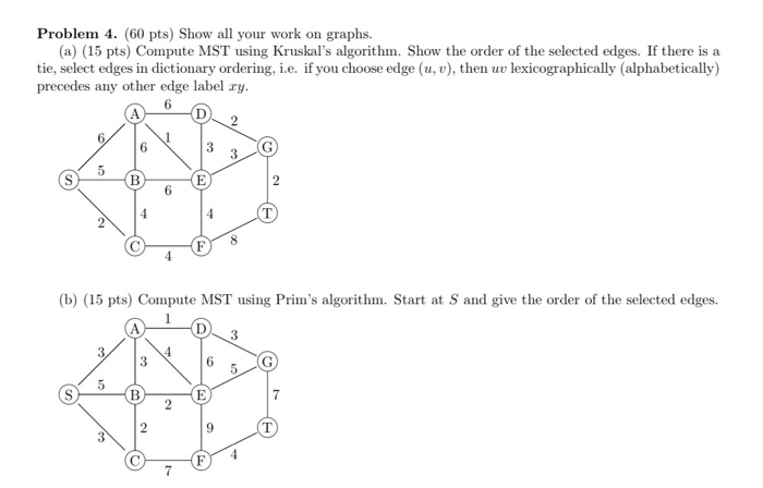
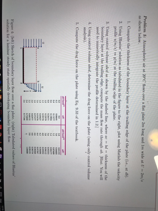
Problem 4. (60 pts) Show all your work on graphs. (a) (15 pts) Compute MST using Kruskal's algorithm. Show the order of the selected edges. If there is a tie, select edges in dictionary ordering, i.e. if you choose edge (u, v), then uv lexicographically (alphabetically) precedes any other edge label ry. 6 A D 2 6 6 3 3 5 B E 6 4 4 F 19 (b) (15 pts) Compute MST using Prim's algorithm. Start at S and give the order of the selected edges. 3, A D S 3 . 6 5 B E 2 2 9 T F 7 = 2m/s Problem 5: Atmospheric air at 20C flows over a flat plate 2m long and 1m wide at U = as shown below. 1. Compute the thickness of the boundary layer at the trailing edge of the plate (i.e., at db). 2. Using Blasius' solution as tabulated in the figure to the right, plot using Matlab the velocity profile u(m/s) vs y(m) at the trailing edge of the plate. 3. Using control volume abcd as shown by the dashed line, where ac = bd thickness of the boundary layer at the trailing edge, compute the mass flow rate through ab. [Hint: You will need to numerically integrate the profile determined in 1.2.] 4. Using control volume abcd, determine the drag force on the plate (using only control volume analysis). 5. Compute the drag force on the plate using Eq. 9.33 of the textbook. WU 0.0 0.0 28 081152 0.2 0.06641 3.0 084605 0.4 0.13277 32 0.87609 0.6 0.19894 3.4 090177 0.8 0.26471 3.6 092333 10 0.32979 3.8 0.94112 12 0.39378 4.0 0.95552 14 0.45627 4.2 0.96696 1.6 0.51676 4.4 097587 1.8 0.57477 4.6 098269 2.0 0.62977 4.8 098779 2.2 0.68132 5.0 099155 24 0.72899 100000 2.6 0.77246 Figure 4: (left) Sketch of boundary layer flow over a flat plate. (right) Tabulated values of Blasius' solution for a laminar steady state spatially developing boundary layer flow. 12:10