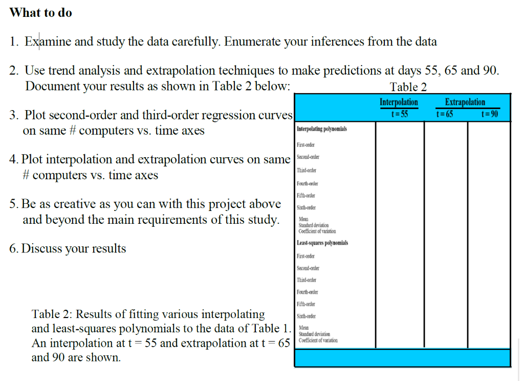
Problem Statement As an engineer with the Ultimate Company you are provided with the following measured data: Table 1 Number of Computers on the 50.000 Market as a function of time Time, Number of Computers days on the Market 0 50,000 10 35,000 20 31,000 30 20,000 40 19,000 50 12,050 60 11,000 Timu, days Number of computati Figure 1. Number of Computers on the Market versus Time. What to do 1. Examine and study the data carefully. Enumerate your inferences from the data 2. Use trend analysis and extrapolation techniques to make predictions at days 55, 65 and 90. Document your results as shown in Table 2 below: Table 2 Interpolation Extrapolation 3. Plot second-order and third-order regression curves t=90 on same #computers vs. time axes t = 55 t=65 Interpolating polynomials First-order Second-order 4. Plot interpolation and extrapolation curves on same # computers vs. time axes Third-order Fourth-order Fifth-order Sixth-order 5. Be as creative as you can with this project above and beyond the main requirements of this study. Mean Standard deviation Coefficient of variation 6. Discuss your results Least-squares polynomials First-order Second-order Third-order Fourth-order Fifth-order Sixth-order Table 2: Results of fitting various interpolating and least-squares polynomials to the data of Table 1. Men An interpolation at t= 55 and extrapolation at t = 65 Coelie of variativa and 90 are shown. Standard deviation Problem Statement As an engineer with the Ultimate Company you are provided with the following measured data: Table 1 Number of Computers on the 50.000 Market as a function of time Time, Number of Computers days on the Market 0 50,000 10 35,000 20 31,000 30 20,000 40 19,000 50 12,050 60 11,000 Timu, days Number of computati Figure 1. Number of Computers on the Market versus Time. What to do 1. Examine and study the data carefully. Enumerate your inferences from the data 2. Use trend analysis and extrapolation techniques to make predictions at days 55, 65 and 90. Document your results as shown in Table 2 below: Table 2 Interpolation Extrapolation 3. Plot second-order and third-order regression curves t=90 on same #computers vs. time axes t = 55 t=65 Interpolating polynomials First-order Second-order 4. Plot interpolation and extrapolation curves on same # computers vs. time axes Third-order Fourth-order Fifth-order Sixth-order 5. Be as creative as you can with this project above and beyond the main requirements of this study. Mean Standard deviation Coefficient of variation 6. Discuss your results Least-squares polynomials First-order Second-order Third-order Fourth-order Fifth-order Sixth-order Table 2: Results of fitting various interpolating and least-squares polynomials to the data of Table 1. Men An interpolation at t= 55 and extrapolation at t = 65 Coelie of variativa and 90 are shown. Standard deviation