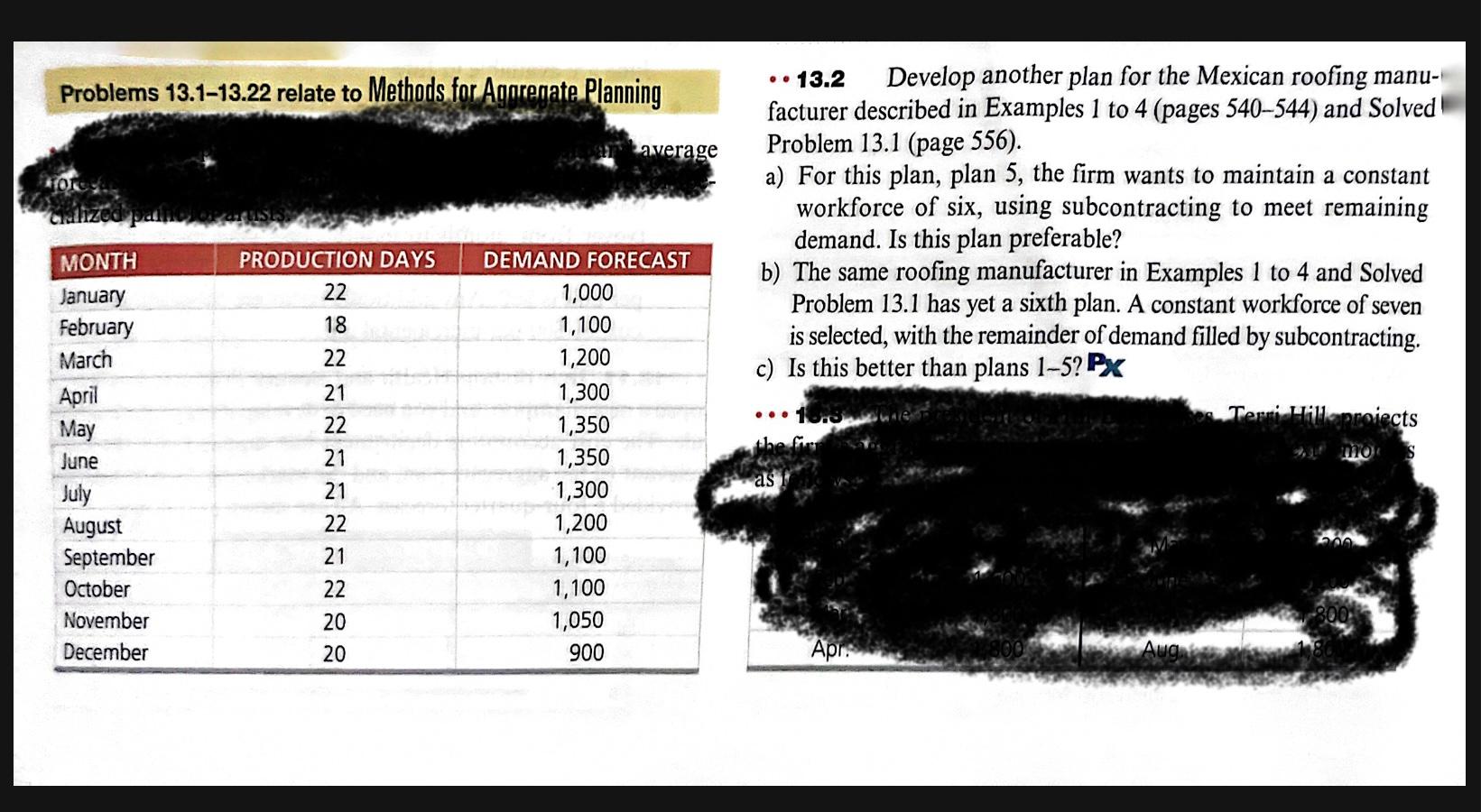
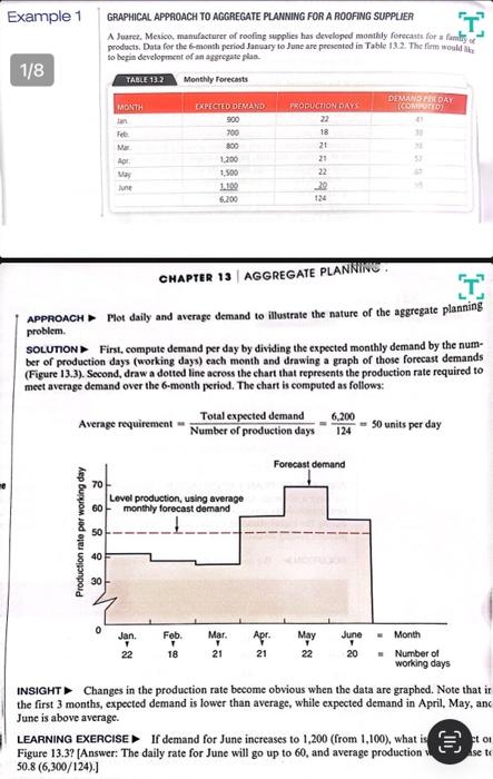
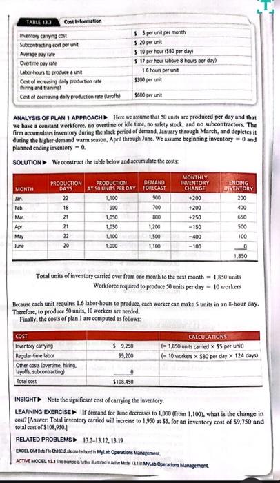
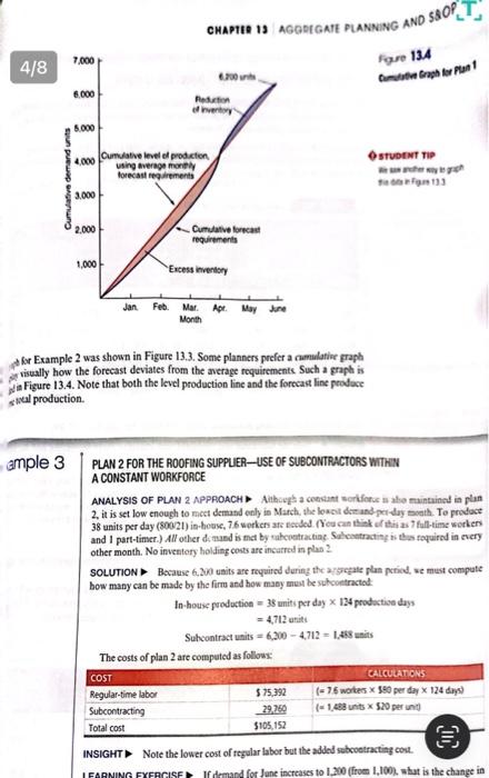
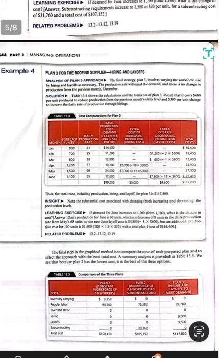
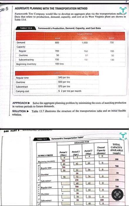
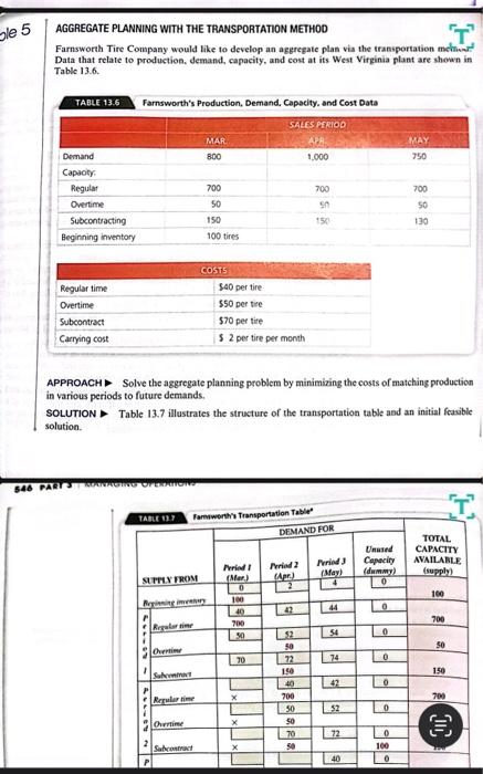
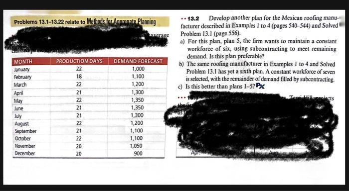
Problems 13.1-13.22 relate to Methods for Agnrejate. Planning -13.2 Develop another plan for the Mexican roofing manufacturer described in Examples 1 to 4 (pages 540-544) and Solved Problem 13.1 (page 556). a) For this plan, plan 5, the firm wants to maintain a constant workforce of six, using subcontracting to meet remaining demand. Is this plan preferable? b) The same roofing manufacturer in Examples 1 to 4 and Solved Problem 13.1 has yet a sixth plan. A constant workforce of seven is selected, with the remainder of demand filled by subcontracting. c) Is this better than plans 15 ? PX Example 1 GRAPHICAL APPROACH TO AGGREGATE PLANING FOR A ROOFING SUPPUER A Juarez. Mesico, mamufacturer of roofing supplics has developod monthly forecasts for a farniry of = ? prodocts. Dat for the 6-month period January to June are prosented in Table 132. The firm would akte to bepia development ed an aggregate plaa. 1/8 CHAPTER 13 AGGREGATE PLANNINU. APPROACH - Mot daily and average demand to illustrate the nature of the aggregate planning problem. soLUnON - First, compate demand per day by dividing the expected monthly demand by the number of production days (working days) each month and drawing a graph of those forecast demands (Figure 13.3). Second, draw a dotted line across the chart that represents the production rate required to meet average demand over the 6-month period. The chart is computed as follows: Average requirement =NumberofproductiondaysTotalexpecteddemand=1246.200=50 units per day INSIGHT - Changes in the production rate become obvious when the data are graphed. Note that it the first 3 months, expected demand is lower than average, while expected demand in April, May, anc June is above average. LEARNING EXERCISE If demand for June increases to 1,200 (from 1,100), what is r ) to Figure 13.3? [Answer: The daily rate for June will go up to 60 , and average production 4 , Ise to 50.8(6,300/124)] ] ANALYSIS OF PLAN I APPAOACH \& Here we assume that $0 units are produced per day and that we have a constast workforet, no overtime of ille lime, no saftly stock, and no subcontractors. The firm accumblases investory during the slack period of demand, January through March, and depletes it during the higher-demand warm seasoo, Apeil throogh June. We assume beginning inventory =0 and planscd ending ieventory =0. SOLUTION We construct the table below and accumulate the costs: Total units of ieventory carried over from one moeth to the sext month =1,850 units Workforce required to produce 50 units per day =10 workers Because each unit require 1.6 labor-hoers to produce, each worker can make 5 units in an 8-hour day. Thertfore, to produce 50 units, 10 workers are netded. Finally, the costs of plan 1 are computed as follows: INSIGHT Note the significent cost of carrying the isventory. LEARNING ECERCISE If demand for Juse decreases to 1,000 (from 1,100), what is the change in cos? [Answer: Total inventory carritd will increase to 1,950 at $5, for an iaventory cost of $9,750 and total cost of $108,930. RELATED PROBLEMS 13.2-13.12, 13.19 Bucel cu Don fli Guene det tan be lart in MyLab operators Manegement cHAPTE is AGODTGAIE PLANNING AND 53OL. 4/8 Fare 134 cimesten toph tor funt 1 Ostubem nie fiaserian 113 tor Example 2 was shown in Figure 13.3. Some planners prefer a camulative graph grisullly how the foreeast deviates from the average requirements Such a graph is Piofigure 13.4. Note that both the level production line and the forecast line peodoce shal production. ample 3 PLAN 2 FOR THE ROOFIG SUPPUER-USE OF SUBCONTRACTORS WITIN A CONSTANT WORKFORCE other month. No inventery holiding cons are incurtral in plas ? SoLumion - Because 6,200 units ane nequired during the argetale plan priod, we must compute bow many can be made by the firm and how macy mol be eriforetractod. InhousproductionSulvontractunits=35unitiperday134podectivedys=4,712uritt=6,2004,712=1,asmaits The costs of plan 2 are computed as follow: INSIGHT - Note the lower cost of tegular labor but the added sabcoutncting cone. LEAPNING EXEACISE If demand lor Jwhe a tht cost? [Answer: Subcontracting requirements increase to 1,508 at 520 per unit, for a subcontracting cost of $31,760 and a total cost of $107,152. RELATED PAOBLEMS 13.213.12,13.19 MANAGING OPCRATIONS 4 PLAN 3 FOA THE AOOFING SUPPUER-HRAN ANO LEOFFS Prodaction flem the perwios noed. Decoller. to intere the dally rate of productien dropl hirep. Thes, the toenl cost, induling production, liting and lugot, for plan 3 in 5117,100 peoduction levelh cest? [Anwwer Daily prodution for June is 6 anith which in derrase of t wnit in the daily preciction RELATED PAOOLEMS 13.2-13.12.11.1 The final step in the graphical metbod is to compare the cons of each peoposed plan and to select the appeoach with the least total cout. A wenmary aadyuis is provided in Table 13.5. We see that because plan 2 has the lowest cont, it is the best of the three options. AGGREGATE PLANNING WITH THE TRANSPORTATION METHOO Farnsworth Tire Company would like to develop an aggrepate plan via the transportation methind? Data that relate to production, demand, capacity, and cost at its Wea Virginia plant are shown in Table 13.6. APPAOACH Solve the aggregate planning problem by minimixing the costs of matching production in various periods to future demands. SOLUTION > Table 13.7 illestrates the structure of the transportation table and an initial fcasible solution. AGGREGATE PLANNING WITH THE TRANSPORTATION METHOD Farnsworth Tire Company would like to develop an aggregate plan via the transportation methind? Data that relate to production. demand, capacity, and cost at its West Virginia plant are shown in Table 13.6. APPROACH Solve the aggregate planning problem by minimizing the costs of matching production in various periods to future demands. SOLUTION - Table 13.7 illustrates the structure of the transportation table and an initial fcasible solution. Problems 13.1-13.22 relate to Methods for-Agnrenate. Planning 13.2 Develop another plan for the Mexican roofing manufacturer described in Examples 1 to 4 (pages 540-544) and Solved Problem 13.1 (page 556). a) For this plan, plan 5 , the firm wants to maintain a constant workforce of six, using subcontracting to meet remaining demand. Is this plan preferable? b) The same roofing manufacturer in Examples 1 to 4 and Solved Problem 13.1 has yet a sixth plan. A constant workforce of seven is selected, with the remainder of demand filled by subcontracting. c) Is this better than plans 1-5? Px Problems 13.1-13.22 relate to Methods for Agnrejate. Planning -13.2 Develop another plan for the Mexican roofing manufacturer described in Examples 1 to 4 (pages 540-544) and Solved Problem 13.1 (page 556). a) For this plan, plan 5, the firm wants to maintain a constant workforce of six, using subcontracting to meet remaining demand. Is this plan preferable? b) The same roofing manufacturer in Examples 1 to 4 and Solved Problem 13.1 has yet a sixth plan. A constant workforce of seven is selected, with the remainder of demand filled by subcontracting. c) Is this better than plans 15 ? PX Example 1 GRAPHICAL APPROACH TO AGGREGATE PLANING FOR A ROOFING SUPPUER A Juarez. Mesico, mamufacturer of roofing supplics has developod monthly forecasts for a farniry of = ? prodocts. Dat for the 6-month period January to June are prosented in Table 132. The firm would akte to bepia development ed an aggregate plaa. 1/8 CHAPTER 13 AGGREGATE PLANNINU. APPROACH - Mot daily and average demand to illustrate the nature of the aggregate planning problem. soLUnON - First, compate demand per day by dividing the expected monthly demand by the number of production days (working days) each month and drawing a graph of those forecast demands (Figure 13.3). Second, draw a dotted line across the chart that represents the production rate required to meet average demand over the 6-month period. The chart is computed as follows: Average requirement =NumberofproductiondaysTotalexpecteddemand=1246.200=50 units per day INSIGHT - Changes in the production rate become obvious when the data are graphed. Note that it the first 3 months, expected demand is lower than average, while expected demand in April, May, anc June is above average. LEARNING EXERCISE If demand for June increases to 1,200 (from 1,100), what is r ) to Figure 13.3? [Answer: The daily rate for June will go up to 60 , and average production 4 , Ise to 50.8(6,300/124)] ] ANALYSIS OF PLAN I APPAOACH \& Here we assume that $0 units are produced per day and that we have a constast workforet, no overtime of ille lime, no saftly stock, and no subcontractors. The firm accumblases investory during the slack period of demand, January through March, and depletes it during the higher-demand warm seasoo, Apeil throogh June. We assume beginning inventory =0 and planscd ending ieventory =0. SOLUTION We construct the table below and accumulate the costs: Total units of ieventory carried over from one moeth to the sext month =1,850 units Workforce required to produce 50 units per day =10 workers Because each unit require 1.6 labor-hoers to produce, each worker can make 5 units in an 8-hour day. Thertfore, to produce 50 units, 10 workers are netded. Finally, the costs of plan 1 are computed as follows: INSIGHT Note the significent cost of carrying the isventory. LEARNING ECERCISE If demand for Juse decreases to 1,000 (from 1,100), what is the change in cos? [Answer: Total inventory carritd will increase to 1,950 at $5, for an iaventory cost of $9,750 and total cost of $108,930. RELATED PROBLEMS 13.2-13.12, 13.19 Bucel cu Don fli Guene det tan be lart in MyLab operators Manegement cHAPTE is AGODTGAIE PLANNING AND 53OL. 4/8 Fare 134 cimesten toph tor funt 1 Ostubem nie fiaserian 113 tor Example 2 was shown in Figure 13.3. Some planners prefer a camulative graph grisullly how the foreeast deviates from the average requirements Such a graph is Piofigure 13.4. Note that both the level production line and the forecast line peodoce shal production. ample 3 PLAN 2 FOR THE ROOFIG SUPPUER-USE OF SUBCONTRACTORS WITIN A CONSTANT WORKFORCE other month. No inventery holiding cons are incurtral in plas ? SoLumion - Because 6,200 units ane nequired during the argetale plan priod, we must compute bow many can be made by the firm and how macy mol be eriforetractod. InhousproductionSulvontractunits=35unitiperday134podectivedys=4,712uritt=6,2004,712=1,asmaits The costs of plan 2 are computed as follow: INSIGHT - Note the lower cost of tegular labor but the added sabcoutncting cone. LEAPNING EXEACISE If demand lor Jwhe a tht cost? [Answer: Subcontracting requirements increase to 1,508 at 520 per unit, for a subcontracting cost of $31,760 and a total cost of $107,152. RELATED PAOBLEMS 13.213.12,13.19 MANAGING OPCRATIONS 4 PLAN 3 FOA THE AOOFING SUPPUER-HRAN ANO LEOFFS Prodaction flem the perwios noed. Decoller. to intere the dally rate of productien dropl hirep. Thes, the toenl cost, induling production, liting and lugot, for plan 3 in 5117,100 peoduction levelh cest? [Anwwer Daily prodution for June is 6 anith which in derrase of t wnit in the daily preciction RELATED PAOOLEMS 13.2-13.12.11.1 The final step in the graphical metbod is to compare the cons of each peoposed plan and to select the appeoach with the least total cout. A wenmary aadyuis is provided in Table 13.5. We see that because plan 2 has the lowest cont, it is the best of the three options. AGGREGATE PLANNING WITH THE TRANSPORTATION METHOO Farnsworth Tire Company would like to develop an aggrepate plan via the transportation methind? Data that relate to production, demand, capacity, and cost at its Wea Virginia plant are shown in Table 13.6. APPAOACH Solve the aggregate planning problem by minimixing the costs of matching production in various periods to future demands. SOLUTION > Table 13.7 illestrates the structure of the transportation table and an initial fcasible solution. AGGREGATE PLANNING WITH THE TRANSPORTATION METHOD Farnsworth Tire Company would like to develop an aggregate plan via the transportation methind? Data that relate to production. demand, capacity, and cost at its West Virginia plant are shown in Table 13.6. APPROACH Solve the aggregate planning problem by minimizing the costs of matching production in various periods to future demands. SOLUTION - Table 13.7 illustrates the structure of the transportation table and an initial fcasible solution. Problems 13.1-13.22 relate to Methods for-Agnrenate. Planning 13.2 Develop another plan for the Mexican roofing manufacturer described in Examples 1 to 4 (pages 540-544) and Solved Problem 13.1 (page 556). a) For this plan, plan 5 , the firm wants to maintain a constant workforce of six, using subcontracting to meet remaining demand. Is this plan preferable? b) The same roofing manufacturer in Examples 1 to 4 and Solved Problem 13.1 has yet a sixth plan. A constant workforce of seven is selected, with the remainder of demand filled by subcontracting. c) Is this better than plans 1-5? Px