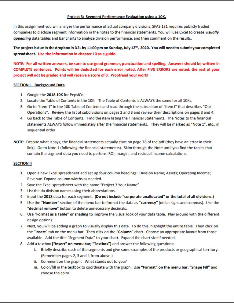
Project 3: Segment Performance Evaluation using a 10K. In this assignment you will analyze the performance of actual company divisions. SFAS 131 requires publicly traded companies to disclose segment information in the notes to the financial statements. You will use Excel to create visually appealing data tables and bar charts to analyze division performance, and then comment on the results. The project is due in the dropbox in D2L by 11:00 pm on Sunday, July 12th, 2020. You will need to submit your completed spreadsheet. Use the information in chapter 10 as a guide. NOTE: For all written answers, be sure to use good grammar, punctuation and spelling. Answers should be written in COMPLETE sentences. Points will be deducted for each error noted. After FIVE ERRORS are noted, the rest of your project will not be graded and will receive a score of 0. Proofread your work! SECTION I - Background Data 1. Google the 2018 10K for PepsiCo. 2. Locate the Table of Contents in the 10K. The Table of Contents is ALWAYS the same for all 10KS. 3. Go to "item 1" in the 10K Table of Contents and read through the subsection of "ItemI" that describes "Our Operations". Review the list of subdivisions on pages 2 and 3 and review their descriptions on pages 3 and 4. 4 Go back to the Table of Contents. Find the item listing the Financial Statements. The Notes to the financial statements ALWAYS follow immediately after the financial statements. They will be marked as "Note 1", etc., in sequential order. NOTE: Despite what it says, the financial statements actually start on page 78 of the pdf (they have an error in their link). Go to Note 1 (following the financial statements). Skim through the Note until you find the tables that contain the segment data you need to perform ROI, margin, and residual income calculations. SECTION II 1. Open a new Excel spreadsheet and set up four column headings: Division Name; Assets; Operating Income; Revenue. Expand column widths as needed. 2. Save the Excel spreadsheet with the name "Project 3 Your Name". 3. List the six division names using their abbreviations. 4. Input the 2018 data for each segment. (Do not include "corporate unallocated" or the total of all divisions.) 5. Use the "Number" section of the menu bar to format the data as "currency" (dollar signs and commas). Use the "decimal remove" button to delete unnecessary decimals. 6. Use "Format as a Table" or shading to improve the visual look of your data table. Play around with the different design options. 7. Next, you will be adding a graph to visually display this data. To do this, highlight the entire table. Then click on the "insert" tab on the menu bar. Then click on the "Column" chart. Choose an appropriate layout from those available. Add the title "Segment Data" to your chart. Expand the chart size if needed. 8. Add a textbox ("Insert" on menu bar; "Textbox") and answer the following questions: i. Briefly describe each of the segments and give some examples of the products or geographical territory. (Remember pages 2, 3 and 4 from above.) ii. Comment on the graph: What stands out to you? ili. Color/fill in the textbox to coordinate with the graph. Use "Format" on the menu bar; "Shape Fill" and choose the color. Project 3: Segment Performance Evaluation using a 10K. In this assignment you will analyze the performance of actual company divisions. SFAS 131 requires publicly traded companies to disclose segment information in the notes to the financial statements. You will use Excel to create visually appealing data tables and bar charts to analyze division performance, and then comment on the results. The project is due in the dropbox in D2L by 11:00 pm on Sunday, July 12th, 2020. You will need to submit your completed spreadsheet. Use the information in chapter 10 as a guide. NOTE: For all written answers, be sure to use good grammar, punctuation and spelling. Answers should be written in COMPLETE sentences. Points will be deducted for each error noted. After FIVE ERRORS are noted, the rest of your project will not be graded and will receive a score of 0. Proofread your work! SECTION I - Background Data 1. Google the 2018 10K for PepsiCo. 2. Locate the Table of Contents in the 10K. The Table of Contents is ALWAYS the same for all 10KS. 3. Go to "item 1" in the 10K Table of Contents and read through the subsection of "ItemI" that describes "Our Operations". Review the list of subdivisions on pages 2 and 3 and review their descriptions on pages 3 and 4. 4 Go back to the Table of Contents. Find the item listing the Financial Statements. The Notes to the financial statements ALWAYS follow immediately after the financial statements. They will be marked as "Note 1", etc., in sequential order. NOTE: Despite what it says, the financial statements actually start on page 78 of the pdf (they have an error in their link). Go to Note 1 (following the financial statements). Skim through the Note until you find the tables that contain the segment data you need to perform ROI, margin, and residual income calculations. SECTION II 1. Open a new Excel spreadsheet and set up four column headings: Division Name; Assets; Operating Income; Revenue. Expand column widths as needed. 2. Save the Excel spreadsheet with the name "Project 3 Your Name". 3. List the six division names using their abbreviations. 4. Input the 2018 data for each segment. (Do not include "corporate unallocated" or the total of all divisions.) 5. Use the "Number" section of the menu bar to format the data as "currency" (dollar signs and commas). Use the "decimal remove" button to delete unnecessary decimals. 6. Use "Format as a Table" or shading to improve the visual look of your data table. Play around with the different design options. 7. Next, you will be adding a graph to visually display this data. To do this, highlight the entire table. Then click on the "insert" tab on the menu bar. Then click on the "Column" chart. Choose an appropriate layout from those available. Add the title "Segment Data" to your chart. Expand the chart size if needed. 8. Add a textbox ("Insert" on menu bar; "Textbox") and answer the following questions: i. Briefly describe each of the segments and give some examples of the products or geographical territory. (Remember pages 2, 3 and 4 from above.) ii. Comment on the graph: What stands out to you? ili. Color/fill in the textbox to coordinate with the graph. Use "Format" on the menu bar; "Shape Fill" and choose the color