Project

Using this link, we collected the suspended sediment concentration and discharge observations at

USGS station $12031000$ CHEHALIS RIVER AT PORTER, WA$.$ The following figure shows the location

of the USGS station.

Let's see what these variables are!

Suspended sediment concentration $($SSC$)$ refers to the amount of solid particles that are

suspended in water. These particles can include silt, clay, sand, and other materials. The

concentration is typically expressed in terms of mass or volume of sediment per unit volume of

water. Common units for SSC include milligrams per liter $(m\frac{g}{L})$ or parts per million $($ppm$).$ River

discharge refers to the volume of water flowing through a river channel over a specific period of

time. It is typically measured in cubic meters per second $(\frac{m^3}{s})$ or cubic feet per second $($cfs$).$ River

discharge is a fundamental and important hydrological parameter as it reflects the movement of

water within a river system.

See the dataset in the attached excel file. This data is collected at daily time scale from October

$01,1961,$ to September $29,1971.$ Here is description of the datasets.

Description

Suspended Sediment Concentration $($SSC$),$ milligrams per liter $($mg$/$L$)$

Discharge, cubic feet per second $($cfs$)$

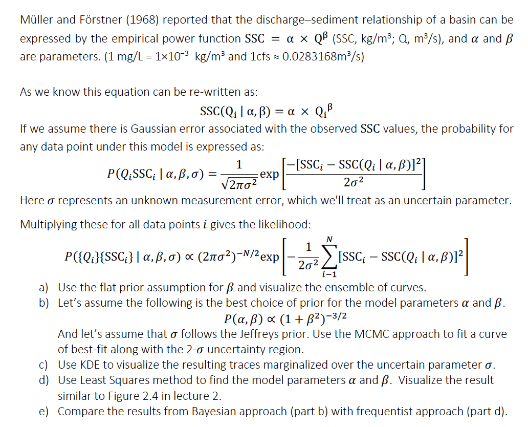
M$$ller and F$$rstner $(1968)$ reported that the discharge$-$sediment relationship of a basin can be

expressed by the empirical power function SSC $=Q^{}($SSC$,\{$:$k\frac{g}{m^3}$;$Q,\frac{m^3}{s}),$ and $$ and $$

are parameters. and $\{$:$1cfs$~~$0\mathrm{.}0283168\frac{m^3}{s})$

As we know this equation can be re$-$written as:

$SSC(Q_i|,)=Q_i^{}$

If we assume there is Gaussian error associated with the observed SSC values, the probability for

any data point under this model is expressed as:

$P(Q_{i}SS{C}_i|,,)=\frac{1}{\sqrt[\phantom{2}]{2{}^2}}$exp$[\frac{-[SS{C}_i-SSC(Q_i|,){]}^2}{2{}^2}]$

Here $$ represents an unknown measurement error, which we'll treat as an uncertain parameter.

Multiplying these for all data points i gives the likelihood:

$P(\{Q_i\}\{SS{C}_i\}|,,)prop(2{}^2{)}^{-\frac{N}{2}}$exp$[-\frac{1}{2{}^2}{\displaystyle \underset{i=1}{\overset{N}{}}}[SS{C}_i-SSC(Q_i|,){]}^2]$

a$)$ Use the flat prior assumption for $$ and visualize the ensemble of curves.

b$)$ Let's assume the following is the best choice of prior for the model parameters $$ and $.$

$P(,)prop(1+{}^2{)}^{-\frac{3}{2}}$

And let's assume that $$ follows the Jeffreys prior. Use the MCMC approach to fit a curve

of best$-$fit along with the $2-$ uncertainty region.

c$)$ Use KDE to visualize the resulting traces marginalized over the uncertain parameter $.$

d$)$ Use Least Squares method to find the model parameters $$ and $.$ Visualize the result

similar to Figure $2\mathrm{.}4$ in lecture $2.$

e$)$ Compare the results from Bayesian approach $($part b$)$ with frequentist approach $($part d$).$