[PYTHON PROGRAMMING]

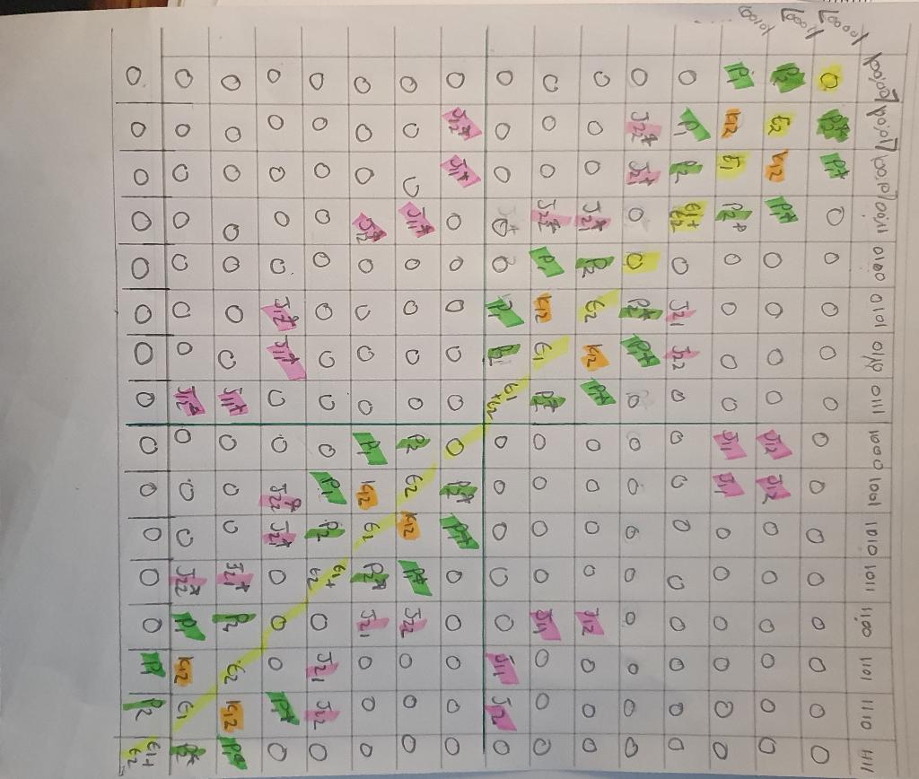
I want to code the hamiltonian matrix given in figure above, in python. In short the hamiltonian describes two systems, the Quantum Network (QN, contaning qubits denoted with sites l) and the computational qubits (denoted as k). Consider the figure below of my hamiltonian for a 2|2 level system, i.e. a 2 QN site with 2 computational qubits, where there are 2 levels. The basis vectors is given as for e.g "00;00", where the first 2 digits are the state of the qubit (0,1) and the last two digits of the QN (2 sites, 0,1). To keep it simple, the E terms determine the energy at site l of QN, the K terms determine the hopping terms between sites, and the J terms determine the coupling between QN sites and computational qubit. 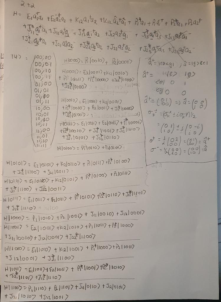The full hamiltonian is as follows figure 3:

I essentially want to code a hamiltonian n by n with dummy variables J,K,E and P which i can replace with real numbers. Also one that I can evolve with time with initial states shown in figure 4 below (ignore the fidelity and density operator stuff, unless if you can provide info on that :D). I really want to check my H and also do larger H's to see patterns for such system. Help would be much appreciated.

For more information on this do read the paper which I am trying to reproduce and learn from: doi:10.1038/s42005-021-00606-3

Thanks!

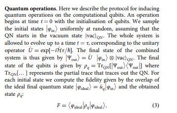
The field operators a^l and a^I are the raising and lowering operators of a two-level system, which can be defined as a^1= egI and a^l=gel, where g and e are the ground and excited states of the system with index l. EI and KI are siteH^QN=lEla^la^l+MKl(a^la^l+a^ dependent energies and nearest-neighbour hopping amplitudes, +(Pta^t+Pla^t). respectively. The last term in Eq. (1) corresponds to the [K0/2], by a classical field. For simplicity we consider a uniform driving, such that Pl=P. All calculations are performed with an open boundary condition (i.e. finite lattice with no periodicity) for the H^=H^QN+kl(Jkl^k+a^l+Jkla^l^^QNHamiltonian.boundarycondition. The QN interacts with a set of computational qubits with the coupling weights Jkb such that the whole system is described by the Hamiltonian H^=H^QN+kl(Jkl^k+a^l+Jkla^l^^k), a^+=(0010)a^=(0100) \begin{tabular}{c|ccccccc|c|c|c|c|c|c|c|c|c} 0 & 0 & 0 & 0 & 0 & 0 & 0 & J128 & 0 & 0 & 0 & J22 & p1 & k12 & 1 & p2 \\ \hline 0 & 0 & 0 & 0 & 0 & 0 & 0 & 0 & 0 & 0 & 0 & 0 & 0 & p2 & p2 & 11 \\ t2 \end{tabular} Quantum operations. Here we describe the protocol for inducing quantum operations on the computational qubits. An operation begins at time t=0 with the initialisation of qubits. We sample the initial states in uniformly at random, assuming that the QN starts in the vacuum state vac}QN. The whole system is allowed to evolve up to a time t=, corresponding to the unitary operator U=exp[iH^/h]. The final state of the combined system is thus given by out=U^invac)QN. The final state of the qubits is given by q=TrQN[outout] where TrQN[] represents the partial trace that traces out the QN. For each initial state we compute the fidelity given by the overlap of the ideal final quantum state ideal=u^qin and the obtained state q F=idealqideal