

Question: python qs, for the echelon qs, someone had asked the similar qs before, but the code didn't work out nicely. I have attached some codes
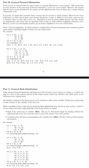
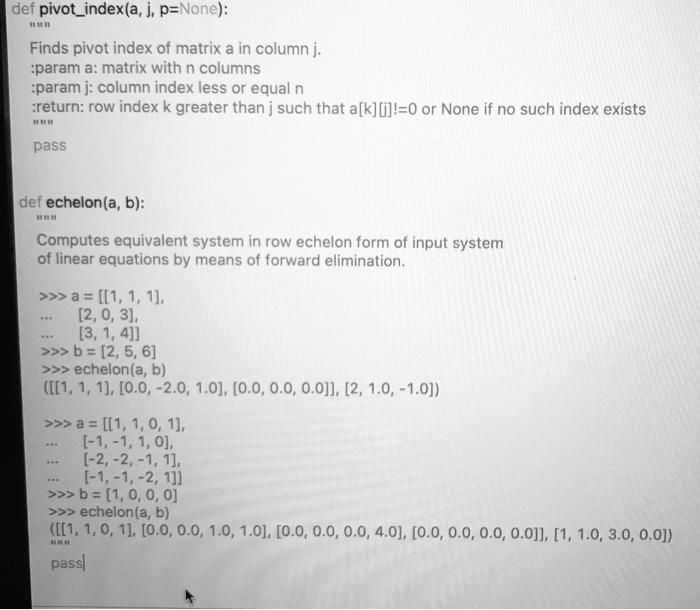
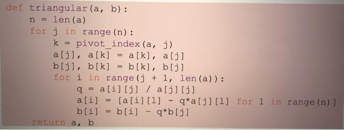
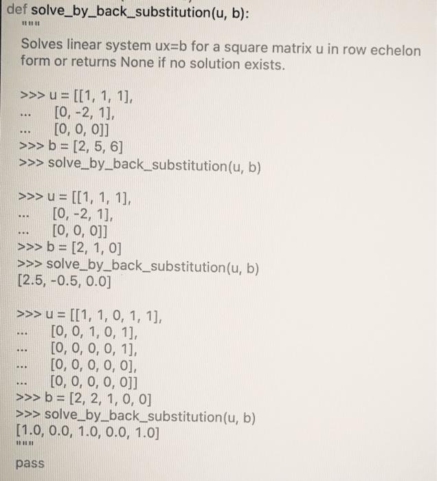


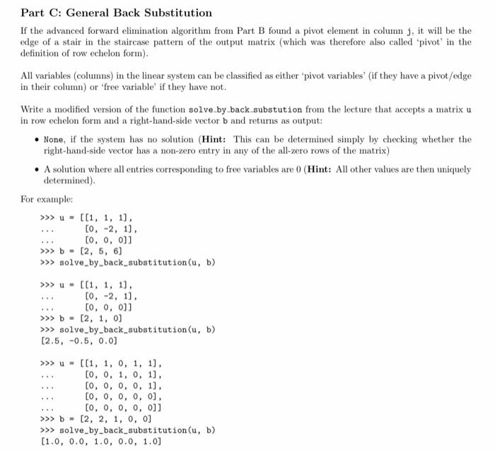
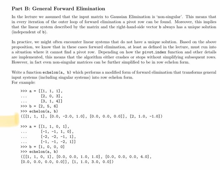

Part B: General Forward Elimination In the stue wed that the matter. This tot was very eat of the fer boup of forward topive well, this that the docted by the matter and he was Independent of b) to presents that do not have to pup, www that in the forward to that were in the man station when it commodi Ding how the pivot ide to other detail At this low apartheither resep withing Howwe in fotot e further simpelthen im Write action call, which is to forward to w (ing) cho For example >>> , 1, 1). 12. 0. 3). 13. 1. 411 >>> 12. 6.6 >>> echella.) (6. 1. 11. 10.0 -2.0, 1.0), 10.0.0.0, 0.091.0.1.0.-1.0) >>> ... 1, , 1). 1-1.-1.1.0). 1-2,-2. -1, 1). >>>> 1.0.0.0 (t. 1. 0. 1). 10.0.0.0, 1.0, 1.0), (0.0.0.0.0.0.4.01. (0.0, 0.0.0.0, 0.01). 1, 1.0, 1.0, 0.01) Part C: General Back Substitution If the files from Partphone, will be the de of star in the pattern of the output matrit (which was called in the det of rowe All riddere Penduta) in the line tu cabe clomited either post variables of the ha perdeler come to output so if the system has to win at: This can be determinat plety shoeking whether the right-handed to try any of the water Abwe allerding to the lake (Hot Atlet values are ded 10.-9. 11. 10.0.0) >>> 12. 5. 6) >>> .I.1). to. -2.11. [, , b >>> 12. 1. ) Whack, white, 12.5, -0.5, 0.01 >> 1. 1. . 1. 11. 1o. . 1. . 1). 10.0.0.1). 10.0...0. 1o. . . .011 >>> 12. 3. 1.0.0 >>> tolv bybackcube, 11.0.0.0, 1.0.0.0, 1.0) def pivot_index(a, j. p=None): Finds pivot index of matrix a in columnj. param a: matrix with n columns param j: column index less or equal n :return: row index k greater than j such that a[k][i]!=0 or None if no such index exists pass def echelon(a, b): Computes equivalent system in row echelon form of input system of linear equations by means of forward elimination. >>> a = [[1, 1, 11, [2.0, 3). [3, 1,4]] >>> b = [2, 5, 6] >>> echelon(a, b) ([[1, 1, 1), (0.0, -2.0, 1.0), (0.0, 0.0, 0.0]], [2, 1.0,-1.0]) >>> a = [[1,1,0, 1], [-1,-1, 1, 0], [-2, -2, -1, 11. [-1,-1, -2, 131 >>> b = (1, 0, 0, 0] >>> echelon(a, b) ([[1,1,0, 1), (0.0, 0.0, 1.0, 1.0), (0.0, 0.0, 0.0, 4.0), (0.0, 0.0, 0.0, 0.0]], [1, 1.0, 3.0, 0.0]) pass def triangular(a, b): n = len(a) for j in range (n): k = pivot_index (a, j) alil, a[k] = a[k], a[j] b[j], b[k] = b[k], b[j] for i in range ( + 1, len(a)): q = a[i][j] / aj][j] a[i] = [a[i] [1] - q*a[i][1] for l in range (n) ] b[i] = b[i] - q*b[j] return a, b def solve_by_back_substitution(u, b): 111111 Solves linear system ux=b for a square matrix u in row echelon form or returns None if no solution exists. >>> u = [[1, 1, 1], [0, -2, 1], [0, 0, 0]] >>> b = [2, 5, 6] >>> solve_by_back_substitution(u, b) . >>> u = [[1, 1, 1] [O, -2, 1], [0, 0, 0]] >>> b = [2, 1, 0] >>> solve_by_back_substitution(u, b) [2.5, -0.5, 0.0] .. . >>> u = [[1, 1, 0, 1, 1], [0, 0, 1, 0, 1], [0, 0, 0, 0, 1], [0, 0, 0, 0, 0], [0, 0, 0, 0, 0]] >>> b = [2, 2, 1, 0, 0] >>> solve_by_back_substitution(u, b) [1.0, 0.0, 1.0, 0.0, 1.0] HII II pass def triangular(a, b): n = len(a) for j in range (n): k = pivot_index (a, j) alil, a[k] = a[k], a[j] b[j], b[k] = b[k], b[j] for i in range ( + 1, len(a)): q = a[i][j] / aj][j] a[i] = [a[i] [1] - q*a[i][1] for l in range (n) ] b[i] = b[i] - q*b[j] return a, b Part B: General Forward Elimination In the lecture we assumed that the input matrix to Gaussian Elimination is non-singular". This means that in every iteration of the outer loop of forward elimination a pivot row can be found. Moreover, this implies that the linear system described by the matrix and the right-hand-side vector b always has a unique solution (independent of b). In practice, we might often encounter linear systems that do not have a unique solution. Based on the above proposition, we know that in these cases forward elimination, at least as defined in the lecture, must run into a situation where it cannot find a pivot row. Depending on how the pivot_index function and other details are implemented, this means that the algorithm either crashes or stops without simplifying subsequent rows. However, in fact even non-singular matrices can be further simplified to be in row echelon form, Write a function echelon(a, b) which performs a modified form of forward elimination that transforms general input systems (including singular systems) into row echelon form. For example: >>> a = [[1, 1, 1), [2, 0, 3), (3, 1, 4)] >>> b - [2, 5, 6) >>> echelon(a, b) ([[1, 1, 1), (0.0, -2.0, 1.0), (0.0, 0.0, 0.0]], [2, 1.0, -1.0]) [[1, 1, 0, 1), [-1,-1, 1, 0] [-2, -2, -1, 1), [-1, -1, -2, 1]] >>> b= (1, 0, 0, 0] >>> echelon(a, b) ([[1, 1, 0, 1), (0.0, 0.0, 1.0, 1.0), (0.0, 0.0, 0.0, 4.0], (0.0, 0.0, 0.0, 0.0]), (1, 1.0, 3.0, 0.0]) Part C: General Back Substitution If the advanced forward elimination algorithm from Part B found a pivot element in column j, it will be the edge of a stair in the staircase pattern of the output matrix (which was therefore also called "pivot' in the definition of row echelon form). All variables (columns) in the linear system can be classified as either pivot variables' (if they have a pivot/edge in their column) or "free variable if they have not. Write a modified version of the function solve by.back substution from the lecture that accepts a matrix u in row echelon form and a right-hand-side vector band returns as output: None, if the system has no solution (Hint: This can be determined simply by checking whether the right-hand-side vector has a non-zero entry in any of the all-zero rows of the matrix) A solution where all entries corresponding to free variables are 0 (Hint: All other values are then uniquely determined). For example: >>> u - ((1, 1, 1). [0, -2, 1) [0, 0, 0]] [2, 5, 6] >>> solve_by_back_substitution (u, b) >>> u - [[1, 1, 1). [0, -2, 1). [0, 0, 0]] >>> b = (2, 1, 0] >>> solve_by_back_substitution (u, b) (2.5, -0.5, 0.0] ... >>> U- [[1, 1, 0, 1, 1], [0, 0, 1, 0, 1). [0, 0, 0, 0, 1). [0, 0, 0, 0, 0], [0, 0, 0, 0, 0]] >>> b- [2, 2, 1, 0, 0] >>> solve_by_back_substitution(u, b) (1.0, 0.0, 1.0, 0.0, 1.0) Part B: General Forward Elimination In the lecture we assumed that the input matrix to Gaussian Elimination is non-singular". This means that in every iteration of the outer loop of forward elimination a pivot row can be found. Moreover, this implies that the linear system described by the matrix and the right-hand-side vector b always has a unique solution (independent of b). In practice, we might often encounter linear systems that do not have a unique solution. Based on the above proposition, we know that in these cases forward elimination, at least as defined in the lecture, must run into a situation where it cannot find a pivot row. Depending on how the pivot_index function and other details are implemented, this means that the algorithm either crashes or stops without simplifying subsequent rows. However, in fact even non-singular matrices can be further simplified to be in row echelon form, Write a function echelon(a, b) which performs a modified form of forward elimination that transforms general input systems (including singular systems) into row echelon form. For example: >>> a = [[1, 1, 1), [2, 0, 3), (3, 1, 4)] >>> b - [2, 5, 6) >>> echelon(a, b) ([[1, 1, 1), (0.0, -2.0, 1.0), (0.0, 0.0, 0.0]], [2, 1.0, -1.0]) [[1, 1, 0, 1), [-1,-1, 1, 0] [-2, -2, -1, 1), [-1, -1, -2, 1]] >>> b= (1, 0, 0, 0] >>> echelon(a, b) ([[1, 1, 0, 1), (0.0, 0.0, 1.0, 1.0), (0.0, 0.0, 0.0, 4.0], (0.0, 0.0, 0.0, 0.0]), (1, 1.0, 3.0, 0.0]) Part C: General Back Substitution If the advanced forward elimination algorithm from Part B found a pivot element in column j, it will be the edge of a stair in the staircase pattern of the output matrix (which was therefore also called "pivot' in the definition of row echelon form). All variables (columns) in the linear system can be classified as either pivot variables' (if they have a pivot/edge in their column) or "free variable if they have not. Write a modified version of the function solve by.back substution from the lecture that accepts a matrix u in row echelon form and a right-hand-side vector band returns as output: None, if the system has no solution (Hint: This can be determined simply by checking whether the right-hand-side vector has a non-zero entry in any of the all-zero rows of the matrix) A solution where all entries corresponding to free variables are 0 (Hint: All other values are then uniquely determined). For example: >>> u - ((1, 1, 1). [0, -2, 1) [0, 0, 0]] [2, 5, 6] >>> solve_by_back_substitution (u, b) >>> u - [[1, 1, 1). [0, -2, 1). [0, 0, 0]] >>> b = (2, 1, 0] >>> solve_by_back_substitution (u, b) (2.5, -0.5, 0.0] ... >>> U- [[1, 1, 0, 1, 1], [0, 0, 1, 0, 1). [0, 0, 0, 0, 1). [0, 0, 0, 0, 0], [0, 0, 0, 0, 0]] >>> b- [2, 2, 1, 0, 0] >>> solve_by_back_substitution(u, b) (1.0, 0.0, 1.0, 0.0, 1.0) Part B: General Forward Elimination In the stue wed that the matter. This tot was very eat of the fer boup of forward topive well, this that the docted by the matter and he was Independent of b) to presents that do not have to pup, www that in the forward to that were in the man station when it commodi Ding how the pivot ide to other detail At this low apartheither resep withing Howwe in fotot e further simpelthen im Write action call, which is to forward to w (ing) cho For example >>> , 1, 1). 12. 0. 3). 13. 1. 411 >>> 12. 6.6 >>> echella.) (6. 1. 11. 10.0 -2.0, 1.0), 10.0.0.0, 0.091.0.1.0.-1.0) >>> ... 1, , 1). 1-1.-1.1.0). 1-2,-2. -1, 1). >>>> 1.0.0.0 (t. 1. 0. 1). 10.0.0.0, 1.0, 1.0), (0.0.0.0.0.0.4.01. (0.0, 0.0.0.0, 0.01). 1, 1.0, 1.0, 0.01) Part C: General Back Substitution If the files from Partphone, will be the de of star in the pattern of the output matrit (which was called in the det of rowe All riddere Penduta) in the line tu cabe clomited either post variables of the ha perdeler come to output so if the system has to win at: This can be determinat plety shoeking whether the right-handed to try any of the water Abwe allerding to the lake (Hot Atlet values are ded 10.-9. 11. 10.0.0) >>> 12. 5. 6) >>> .I.1). to. -2.11. [, , b >>> 12. 1. ) Whack, white, 12.5, -0.5, 0.01 >> 1. 1. . 1. 11. 1o. . 1. . 1). 10.0.0.1). 10.0...0. 1o. . . .011 >>> 12. 3. 1.0.0 >>> tolv bybackcube, 11.0.0.0, 1.0.0.0, 1.0) def pivot_index(a, j. p=None): Finds pivot index of matrix a in columnj. param a: matrix with n columns param j: column index less or equal n :return: row index k greater than j such that a[k][i]!=0 or None if no such index exists pass def echelon(a, b): Computes equivalent system in row echelon form of input system of linear equations by means of forward elimination. >>> a = [[1, 1, 11, [2.0, 3). [3, 1,4]] >>> b = [2, 5, 6] >>> echelon(a, b) ([[1, 1, 1), (0.0, -2.0, 1.0), (0.0, 0.0, 0.0]], [2, 1.0,-1.0]) >>> a = [[1,1,0, 1], [-1,-1, 1, 0], [-2, -2, -1, 11. [-1,-1, -2, 131 >>> b = (1, 0, 0, 0] >>> echelon(a, b) ([[1,1,0, 1), (0.0, 0.0, 1.0, 1.0), (0.0, 0.0, 0.0, 4.0), (0.0, 0.0, 0.0, 0.0]], [1, 1.0, 3.0, 0.0]) pass def triangular(a, b): n = len(a) for j in range (n): k = pivot_index (a, j) alil, a[k] = a[k], a[j] b[j], b[k] = b[k], b[j] for i in range ( + 1, len(a)): q = a[i][j] / aj][j] a[i] = [a[i] [1] - q*a[i][1] for l in range (n) ] b[i] = b[i] - q*b[j] return a, b def solve_by_back_substitution(u, b): 111111 Solves linear system ux=b for a square matrix u in row echelon form or returns None if no solution exists. >>> u = [[1, 1, 1], [0, -2, 1], [0, 0, 0]] >>> b = [2, 5, 6] >>> solve_by_back_substitution(u, b) . >>> u = [[1, 1, 1] [O, -2, 1], [0, 0, 0]] >>> b = [2, 1, 0] >>> solve_by_back_substitution(u, b) [2.5, -0.5, 0.0] .. . >>> u = [[1, 1, 0, 1, 1], [0, 0, 1, 0, 1], [0, 0, 0, 0, 1], [0, 0, 0, 0, 0], [0, 0, 0, 0, 0]] >>> b = [2, 2, 1, 0, 0] >>> solve_by_back_substitution(u, b) [1.0, 0.0, 1.0, 0.0, 1.0] HII II pass def triangular(a, b): n = len(a) for j in range (n): k = pivot_index (a, j) alil, a[k] = a[k], a[j] b[j], b[k] = b[k], b[j] for i in range ( + 1, len(a)): q = a[i][j] / aj][j] a[i] = [a[i] [1] - q*a[i][1] for l in range (n) ] b[i] = b[i] - q*b[j] return a, b Part B: General Forward Elimination In the lecture we assumed that the input matrix to Gaussian Elimination is non-singular". This means that in every iteration of the outer loop of forward elimination a pivot row can be found. Moreover, this implies that the linear system described by the matrix and the right-hand-side vector b always has a unique solution (independent of b). In practice, we might often encounter linear systems that do not have a unique solution. Based on the above proposition, we know that in these cases forward elimination, at least as defined in the lecture, must run into a situation where it cannot find a pivot row. Depending on how the pivot_index function and other details are implemented, this means that the algorithm either crashes or stops without simplifying subsequent rows. However, in fact even non-singular matrices can be further simplified to be in row echelon form, Write a function echelon(a, b) which performs a modified form of forward elimination that transforms general input systems (including singular systems) into row echelon form. For example: >>> a = [[1, 1, 1), [2, 0, 3), (3, 1, 4)] >>> b - [2, 5, 6) >>> echelon(a, b) ([[1, 1, 1), (0.0, -2.0, 1.0), (0.0, 0.0, 0.0]], [2, 1.0, -1.0]) [[1, 1, 0, 1), [-1,-1, 1, 0] [-2, -2, -1, 1), [-1, -1, -2, 1]] >>> b= (1, 0, 0, 0] >>> echelon(a, b) ([[1, 1, 0, 1), (0.0, 0.0, 1.0, 1.0), (0.0, 0.0, 0.0, 4.0], (0.0, 0.0, 0.0, 0.0]), (1, 1.0, 3.0, 0.0]) Part C: General Back Substitution If the advanced forward elimination algorithm from Part B found a pivot element in column j, it will be the edge of a stair in the staircase pattern of the output matrix (which was therefore also called "pivot' in the definition of row echelon form). All variables (columns) in the linear system can be classified as either pivot variables' (if they have a pivot/edge in their column) or "free variable if they have not. Write a modified version of the function solve by.back substution from the lecture that accepts a matrix u in row echelon form and a right-hand-side vector band returns as output: None, if the system has no solution (Hint: This can be determined simply by checking whether the right-hand-side vector has a non-zero entry in any of the all-zero rows of the matrix) A solution where all entries corresponding to free variables are 0 (Hint: All other values are then uniquely determined). For example: >>> u - ((1, 1, 1). [0, -2, 1) [0, 0, 0]] [2, 5, 6] >>> solve_by_back_substitution (u, b) >>> u - [[1, 1, 1). [0, -2, 1). [0, 0, 0]] >>> b = (2, 1, 0] >>> solve_by_back_substitution (u, b) (2.5, -0.5, 0.0] ... >>> U- [[1, 1, 0, 1, 1], [0, 0, 1, 0, 1). [0, 0, 0, 0, 1). [0, 0, 0, 0, 0], [0, 0, 0, 0, 0]] >>> b- [2, 2, 1, 0, 0] >>> solve_by_back_substitution(u, b) (1.0, 0.0, 1.0, 0.0, 1.0) Part B: General Forward Elimination In the lecture we assumed that the input matrix to Gaussian Elimination is non-singular". This means that in every iteration of the outer loop of forward elimination a pivot row can be found. Moreover, this implies that the linear system described by the matrix and the right-hand-side vector b always has a unique solution (independent of b). In practice, we might often encounter linear systems that do not have a unique solution. Based on the above proposition, we know that in these cases forward elimination, at least as defined in the lecture, must run into a situation where it cannot find a pivot row. Depending on how the pivot_index function and other details are implemented, this means that the algorithm either crashes or stops without simplifying subsequent rows. However, in fact even non-singular matrices can be further simplified to be in row echelon form, Write a function echelon(a, b) which performs a modified form of forward elimination that transforms general input systems (including singular systems) into row echelon form. For example: >>> a = [[1, 1, 1), [2, 0, 3), (3, 1, 4)] >>> b - [2, 5, 6) >>> echelon(a, b) ([[1, 1, 1), (0.0, -2.0, 1.0), (0.0, 0.0, 0.0]], [2, 1.0, -1.0]) [[1, 1, 0, 1), [-1,-1, 1, 0] [-2, -2, -1, 1), [-1, -1, -2, 1]] >>> b= (1, 0, 0, 0] >>> echelon(a, b) ([[1, 1, 0, 1), (0.0, 0.0, 1.0, 1.0), (0.0, 0.0, 0.0, 4.0], (0.0, 0.0, 0.0, 0.0]), (1, 1.0, 3.0, 0.0]) Part C: General Back Substitution If the advanced forward elimination algorithm from Part B found a pivot element in column j, it will be the edge of a stair in the staircase pattern of the output matrix (which was therefore also called "pivot' in the definition of row echelon form). All variables (columns) in the linear system can be classified as either pivot variables' (if they have a pivot/edge in their column) or "free variable if they have not. Write a modified version of the function solve by.back substution from the lecture that accepts a matrix u in row echelon form and a right-hand-side vector band returns as output: None, if the system has no solution (Hint: This can be determined simply by checking whether the right-hand-side vector has a non-zero entry in any of the all-zero rows of the matrix) A solution where all entries corresponding to free variables are 0 (Hint: All other values are then uniquely determined). For example: >>> u - ((1, 1, 1). [0, -2, 1) [0, 0, 0]] [2, 5, 6] >>> solve_by_back_substitution (u, b) >>> u - [[1, 1, 1). [0, -2, 1). [0, 0, 0]] >>> b = (2, 1, 0] >>> solve_by_back_substitution (u, b) (2.5, -0.5, 0.0] ... >>> U- [[1, 1, 0, 1, 1], [0, 0, 1, 0, 1). [0, 0, 0, 0, 1). [0, 0, 0, 0, 0], [0, 0, 0, 0, 0]] >>> b- [2, 2, 1, 0, 0] >>> solve_by_back_substitution(u, b) (1.0, 0.0, 1.0, 0.0, 1.0)
Step by Step Solution
There are 3 Steps involved in it

Get step-by-step solutions from verified subject matter experts