[Python]

The goal is to write a code that shows that movement of a particle in a set of 2 helmholtz coils in a 2D animation.

The equation for the magnetic field:

Equation for the force on the particle when in the magnetic field (magnetic force):

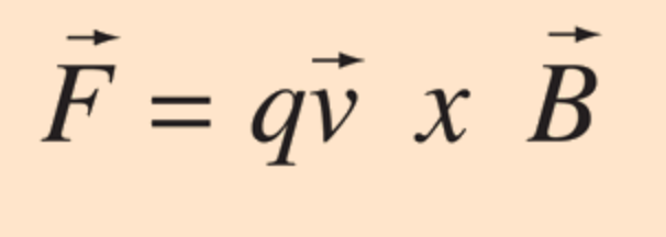
What I have so far (that's not working and not sure how to fix it):

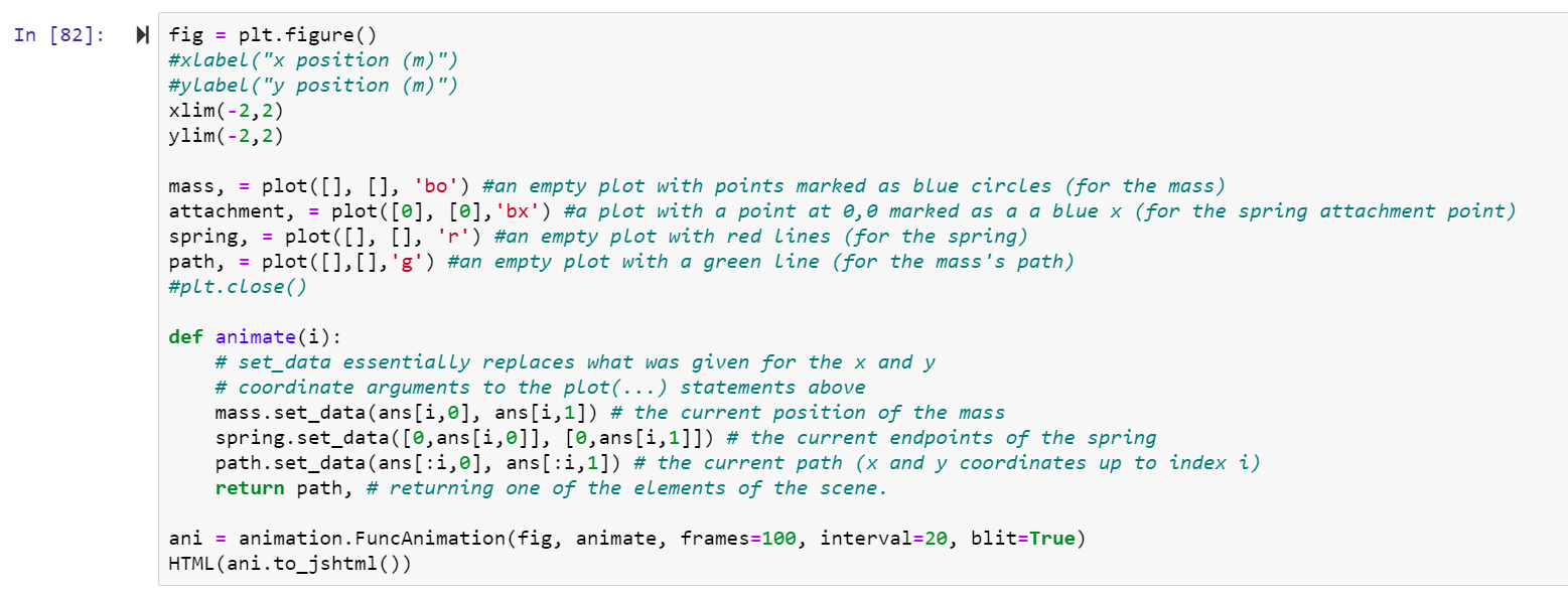
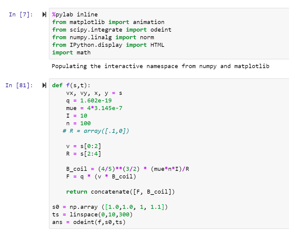Code for the animation, this format and the commands need to be followed:

Any help would be greatly appreciated!!

3/2 400I 4 = 5 R F = q x B In [7]: %pylab inline from matplotlib import animation from scipy.integrate import odeint from numpy.linalg import norm from IPython.display import HTML import math Populating the interactive namespace from numpy and matplotlib In [81]: def f(s, t): VX, vy, x, y = s q = 1.602e-19 mue = 4*3.145e-7 I = 10 n = 100 # R = array([.1,0]) V = s[0:2] R = s[2:4] B_coil = (4/5)** (3/2) (4/5)** (3/2) * (mue*n*I)/R F = q * (v * B_coil) return concatenate([F, B_coil]) SO = np.array ([1.0,1.0, 1, 1.1]) ts = linspace(0, 10,300) ans = odeint(f, so, ts) In [82]: fig = plt. figure() #xLabel("x position (m)") #y Label("y position (m)") xlim(-2,2) ylim(-2,2) mass, = plot([], [], 'bo') #an empty plot with points marked as blue circles (for the mass) attachment, = plot([0], [0], 'bx') #a plot with a point at 0,0 marked as a a blue x (for the spring attachment point) spring, = plot([], [], 'r') #an empty plot with red Lines (for the spring) path, = plot([],[],'g') #an empty plot with a green Line (for the mass's path) #plt.close() def animate(i): # set_data essentially replaces what was given for the x and y # coordinate arguments to the plot(...) statements above mass.set_data(ans[i,0], ans[i,1]) # the current position of the mass spring.set_data([0, ans[i,0]], [0, ans[i,1]]) # the current endpoints of the spring path.set_data(ans[:i,2], ans[:i,1]) # the current path (x and y coordinates to index i) return path, # returning one of the elements of the scene. ani = animation. FuncAnimation(fig, animate, frames=100, interval=20, blit=True) HTML (ani.to_jshtml()) 3/2 400I 4 = 5 R F = q x B In [7]: %pylab inline from matplotlib import animation from scipy.integrate import odeint from numpy.linalg import norm from IPython.display import HTML import math Populating the interactive namespace from numpy and matplotlib In [81]: def f(s, t): VX, vy, x, y = s q = 1.602e-19 mue = 4*3.145e-7 I = 10 n = 100 # R = array([.1,0]) V = s[0:2] R = s[2:4] B_coil = (4/5)** (3/2) (4/5)** (3/2) * (mue*n*I)/R F = q * (v * B_coil) return concatenate([F, B_coil]) SO = np.array ([1.0,1.0, 1, 1.1]) ts = linspace(0, 10,300) ans = odeint(f, so, ts) In [82]: fig = plt. figure() #xLabel("x position (m)") #y Label("y position (m)") xlim(-2,2) ylim(-2,2) mass, = plot([], [], 'bo') #an empty plot with points marked as blue circles (for the mass) attachment, = plot([0], [0], 'bx') #a plot with a point at 0,0 marked as a a blue x (for the spring attachment point) spring, = plot([], [], 'r') #an empty plot with red Lines (for the spring) path, = plot([],[],'g') #an empty plot with a green Line (for the mass's path) #plt.close() def animate(i): # set_data essentially replaces what was given for the x and y # coordinate arguments to the plot(...) statements above mass.set_data(ans[i,0], ans[i,1]) # the current position of the mass spring.set_data([0, ans[i,0]], [0, ans[i,1]]) # the current endpoints of the spring path.set_data(ans[:i,2], ans[:i,1]) # the current path (x and y coordinates to index i) return path, # returning one of the elements of the scene. ani = animation. FuncAnimation(fig, animate, frames=100, interval=20, blit=True) HTML (ani.to_jshtml())