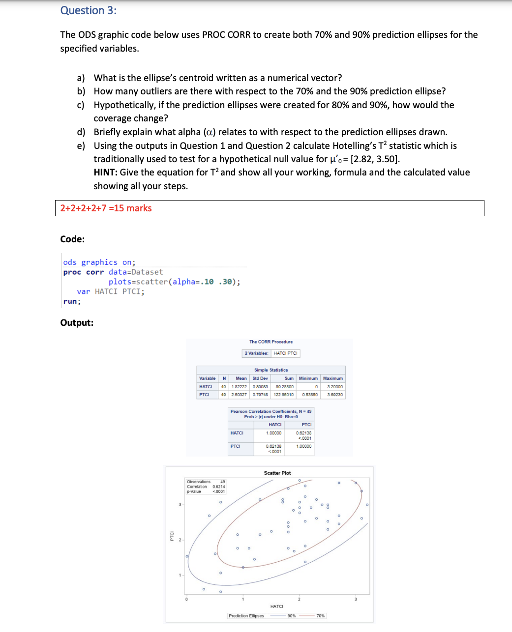
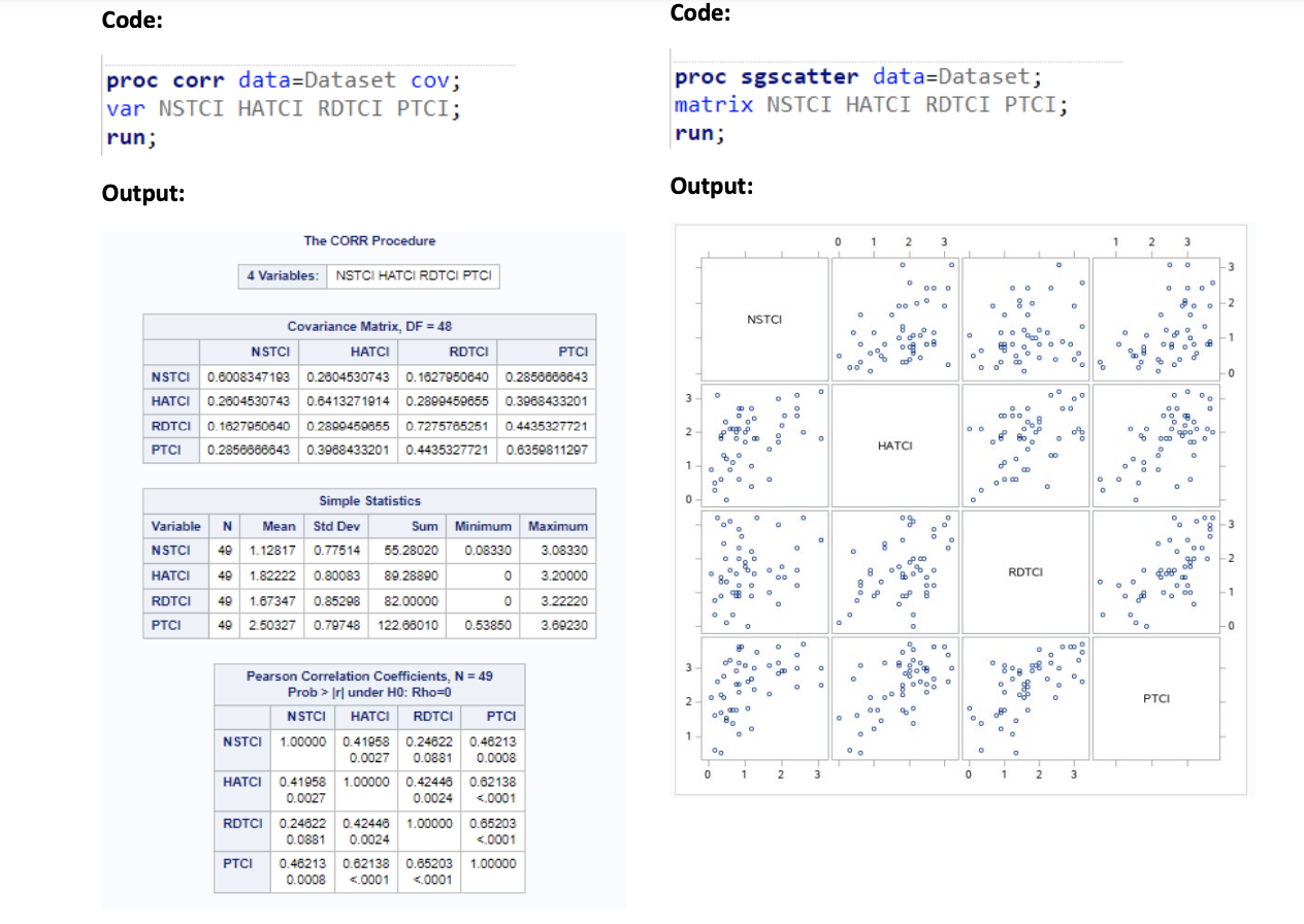
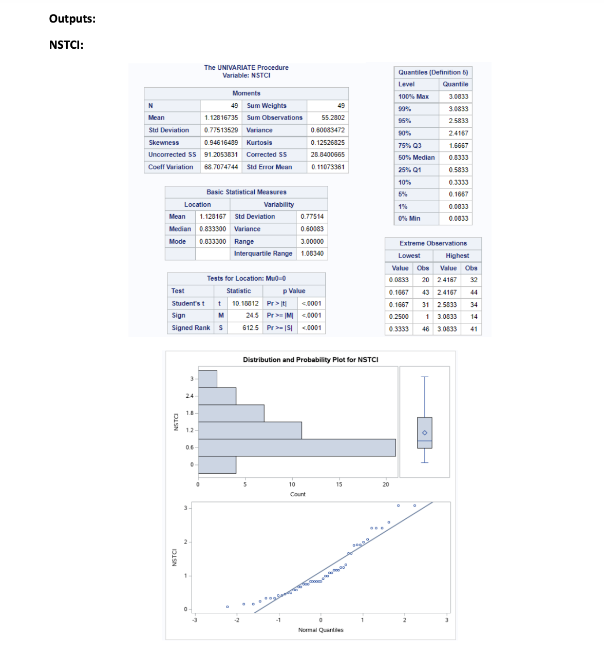
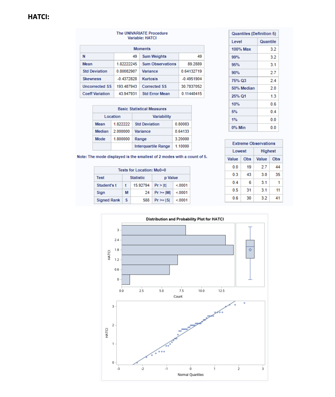
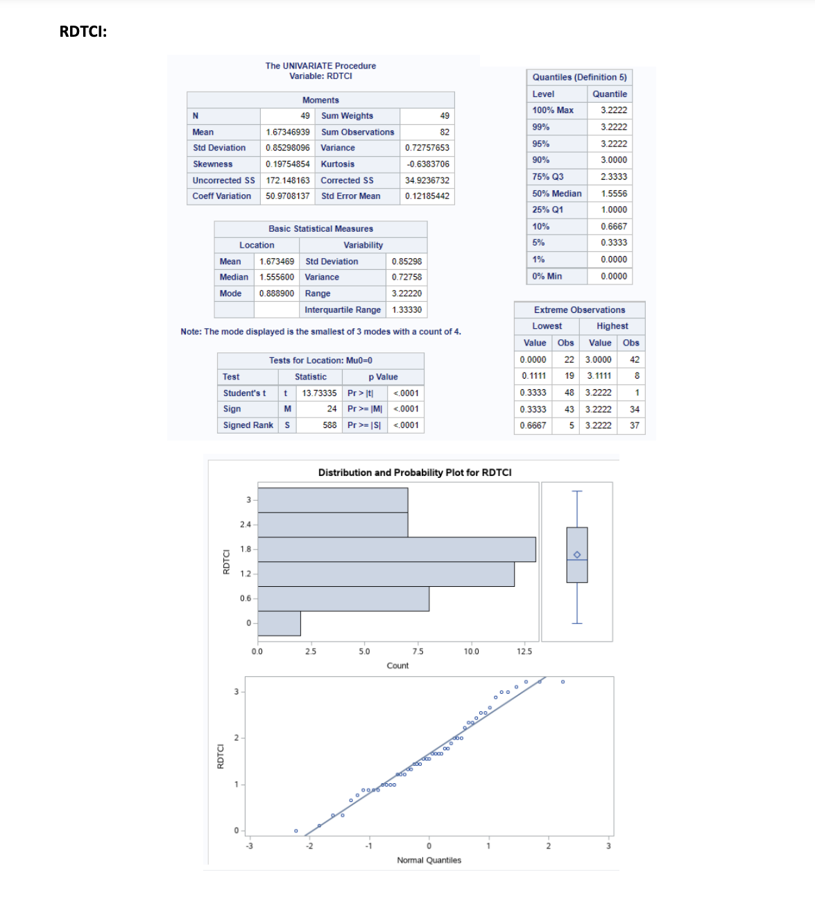
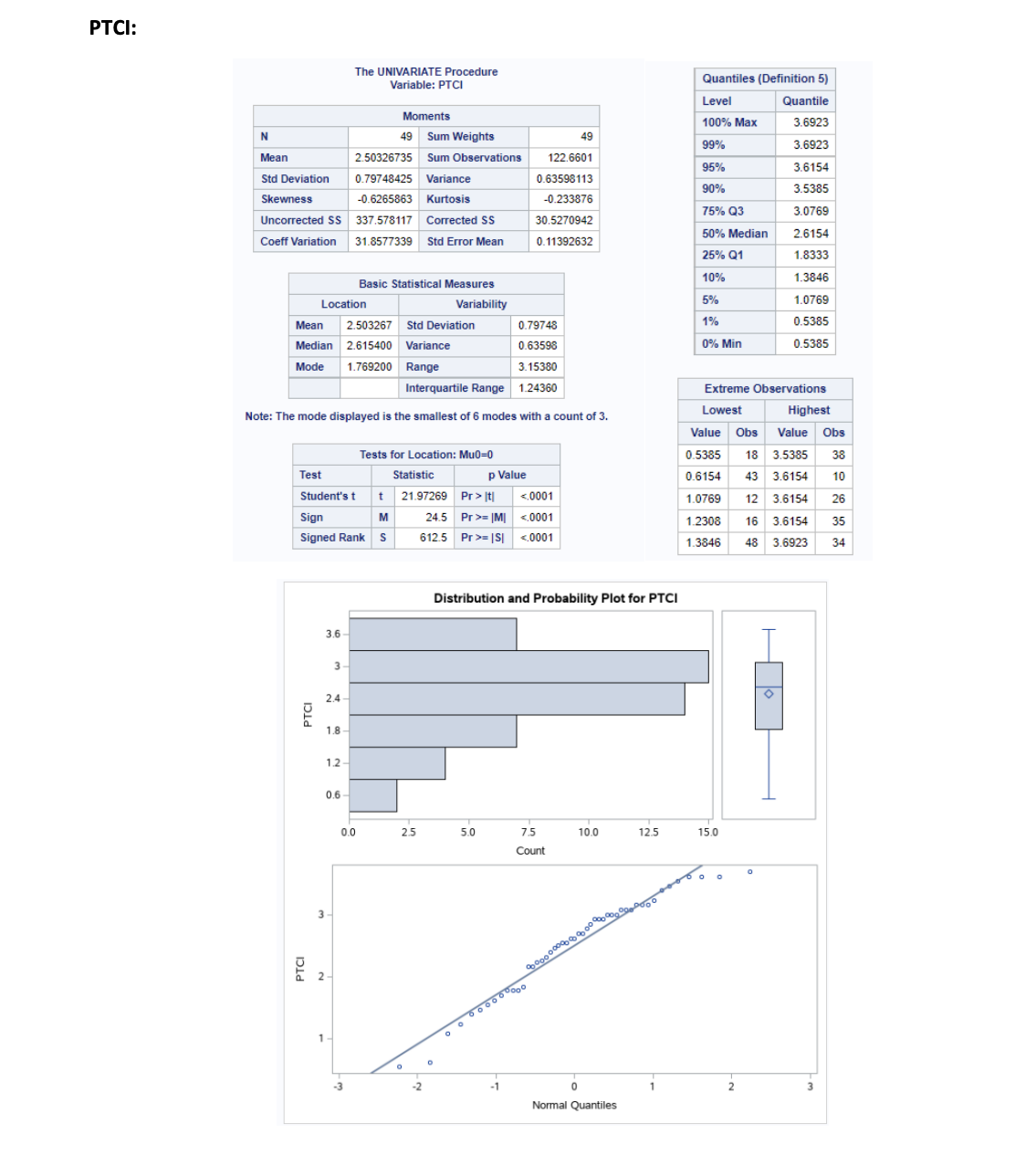
Question 3: The ODS graphic code below uses PROC CORR to create both 70% and 90% prediction ellipses for the specified variables. a) What is the ellipse's centroid written as a numerical vector? b) How many outliers are there with respect to the 70% and the 90% prediction ellipse? c) Hypothetically, if the prediction ellipses were created for 80% and 90%, how would the coverage change? d) Briefly explain what alpha (a) relates to with respect to the prediction ellipses drawn. e) Using the outputs in Question 1 and Question 2 calculate Hotelling's T statistic which is traditionally used to test for a hypothetical null value for 'o[2.82, 3.50]. HINT: Give the equation for T and show all your working, formula and the calculated value showing all your steps. 2+2+2+2+7=15 marks Code: ods graphics on; proc corr data=Dataset plots scatter (alpha=.10.30); var HATCI PTCI; run; Output: g 1 The CORR Procedure 2 Variables: HATCI PTCI Simple Statistics Variable N Mean HATCI 49 1.82222 PTCI Std Dev 0.80083 40 2.50327 0.79748 122.66010 Sum Minimum Maximum 89.28890 3.20000 3.69230 0.53850 Observations Correlation p-Value 0.6214 runder H0: Rho-0 HATCI HATCI 1.00000 PTCI 0.62138 Code: proc corr data=Dataset cov; var NSTCI HATCI RDTCI PTCI; run; Output: Code: proc sgscatter data-Dataset; matrix NSTCI HATCI RDTCI PTCI; run; Output: The CORR Procedure 4 Variables: NSTCI HATCI RDTCI PTCI NSTCI Covariance Matrix, DF = 48 HATCI RDTCI PTCI | NSTCI | 0.6008347183 0.2804530743 0.1627950840 0.2856666643 HATCI 0.2604530743 0.6413271914 0.2899459655 0.3968433201 RDTCI 0.1627950640 0.2899459855 0.7275785251 0.4435327721 PTCI 0.2856666643 0.3968433201 0.4435327721 0.6359811297 Simple Statistics Variable N Mean Std Dev NSTCI 49 1.12817 0.77514 HATCI 49 1.82222 0.80083 RDTCI 49 1.67347 0.85298 PTCI Sum Minimum Maximum 55.28020 0.08330 89.28890 82.00000 0 3.08330 3.20000 0 3.22220 49 2.50327 0.79748 122.66010 0.53850 3.69230 Pearson Correlation Coefficients, N = 49 Prob > Ir] under H0: Rho=0 NSTCI HATCI RDTCI PTCI | NSTC | 1.00000 0.41858 0.24622 0.46213 0.0027 0.0881 0.0008 HATCI 0.41958 1.00000 0.42446 0.62138 0.0027 0.0024 Outputs: NSTCI: N Mean The UNIVARIATE Procedure Variable: NSTCI Moments 49 Sum Weights Quantiles (Definition 5) Level Quantile 100% Max 3.0833 49 99% 3.0833 1.12816735 Sum Observations 55.2802 95% 2.5833 Std Deviation 0.77513529 Variance 0.60083472 90% 2.4167 Skewness Uncorrected SS 0.94616489 Kurtosis 0.12526825 75% Q3 1.6667 Coeff Variation 91.2053831 68.7074744 Corrected SS 28.8400665 50% Median 0.8333 Std Error Mean 0.11073361 25% Q1 0.5833 10% 0.3333 Basic Statistical Measures 5% 0.1667 Location Variability 1% 0.0833 Mean 1.128167 Std Deviation 0.77514 0% Min 0.0833 Median 0.833300 Variance 0.60083 Mode 0.833300 Range 3.00000 Extreme Observations Interquartile Range 1.08340 Lowest Highest Tests for Location: Mu0=0 Test Statistic p Value Student's t t Sign Signed Rank M S 10.18812 Pr> It 24.5 Pr>= |M| 612.5 Pr>= |S| HATCI: N The UNIVARIATE Procedure Variable: HATCI Moments 49 Sum Weights Quantiles (Definition 5) Level Quantile 100% Max 3.2 49 99% 3.2 Mean 1.82222245 Sum Observations 89.2889 95% 3.1 Std Deviation 0.80082907 Variance 0.64132719 90% 2.7 Skewness Uncorrected SS Coeff Variation -0.4372828 Kurtosis 193.487943 Corrected SS 43.947931 Std Error Mean -0.4951904 75% Q3 2.4 30.7837052 50% Median 2.0 0.11440415 25% Q1 1.3 10% 0.6 Basic Statistical Measures 5% 0.4 Location Variability 1% 0.0 Mean 1.822222 Std Deviation Median 2.000000 Variance Mode 0.80083 0% Min 0.0 0.64133 1.800000 Range 3.20000 Extreme Observations Interquartile Range 1.10000 Note: The mode displayed is the smallest of 2 modes with a count of 5. Tests for Location: Mu0=0 Lowest Highest Value Obs Value Obs HATCI 0.0 19 2.7 44 0.3 43 3.0 35 Test Statistic p Value 0.4 6 3.1 1 Student's t Sign t 15.92794 Pr>|t| = |M| = |S| RDTCI: RDTCI N The UNIVARIATE Procedure Variable: RDTCI Moments 49 Sum Weights Quantiles (Definition 5) Level Quantile 100% Max 3.2222 49 99% 3.2222 Mean 1.67346939 Sum Observations 82 95% 3.2222 Std Deviation 0.85298096 Variance 0.72757653 Skewness 0.19754854 90% 3.0000 Kurtosis -0.6383706 75% Q3 2.3333 Uncorrected SS 172.148163 Corrected SS 34.9236732 Coeff Variation 50.9708137 Std Error Mean 0.12185442 50% Median 1.5556 25% Q1 1.0000 10% 0.6667 Basic Statistical Measures Location Mean Variability 5% 0.3333 0.888900 1.673469 Median 1.555600 Variance Mode Std Deviation 0.85298 1% 0.0000 0.72758 0% Min 0.0000 Range Interquartile Range 3.22220 1.33330 Extreme Observations Lowest Highest Note: The mode displayed is the smallest of 3 modes with a count of 4. Tests for Location: Mu0=0 Test Statistic p Value Student's t t 13.73335 Pr>|t| = |M = |S PTCI: PTC 2 The UNIVARIATE Procedure Variable: PTCI Quantiles (Definition 5) Level Quantile N Moments 49 Sum Weights 100% Max 3.6923 49 99% 3.6923 Mean 2.50326735 Sum Observations 122.6601 95% 3.6154 Std Deviation 0.79748425 Variance 0.63598113 90% 3.5385 Skewness -0.6265863 Kurtosis -0.233876 75% Q3 3.0769 Uncorrected SS 337.578117 Corrected SS 30.5270942 50% Median 2.6154 Coeff Variation 31.8577339 Std Error Mean 0.11392632 25% Q1 1.8333 10% 1.3846 Basic Statistical Measures 5% 1.0769 Location Variability 1% Mean 2.503267 Std Deviation 0.79748 0.5385 Median 2.615400 Variance Mode 1.769200 Range 0.63598 0% Min 0.5385 3.15380 Interquartile Range 1.24360 Note: The mode displayed is the smallest of 6 modes with a count of 3. Tests for Location: Mu0=0 Extreme Observations Lowest Highest Value Obs Value Obs 0.5385 18 3.5385 38 0.6154 43 3.6154 10 3 PTCI Test Statistic p Value Student's t t 21.97269 Pr>|t| = |M|| | = |S|