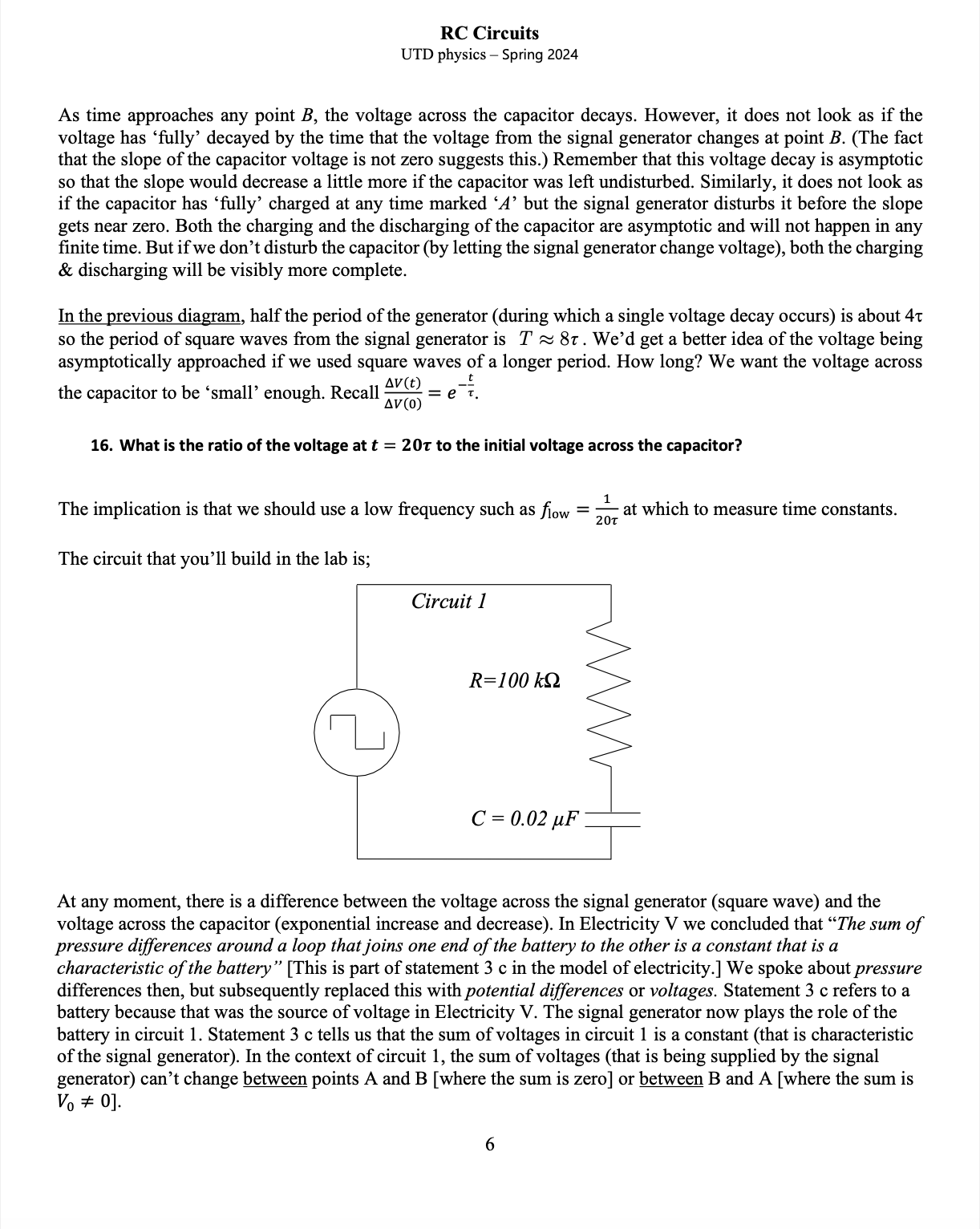
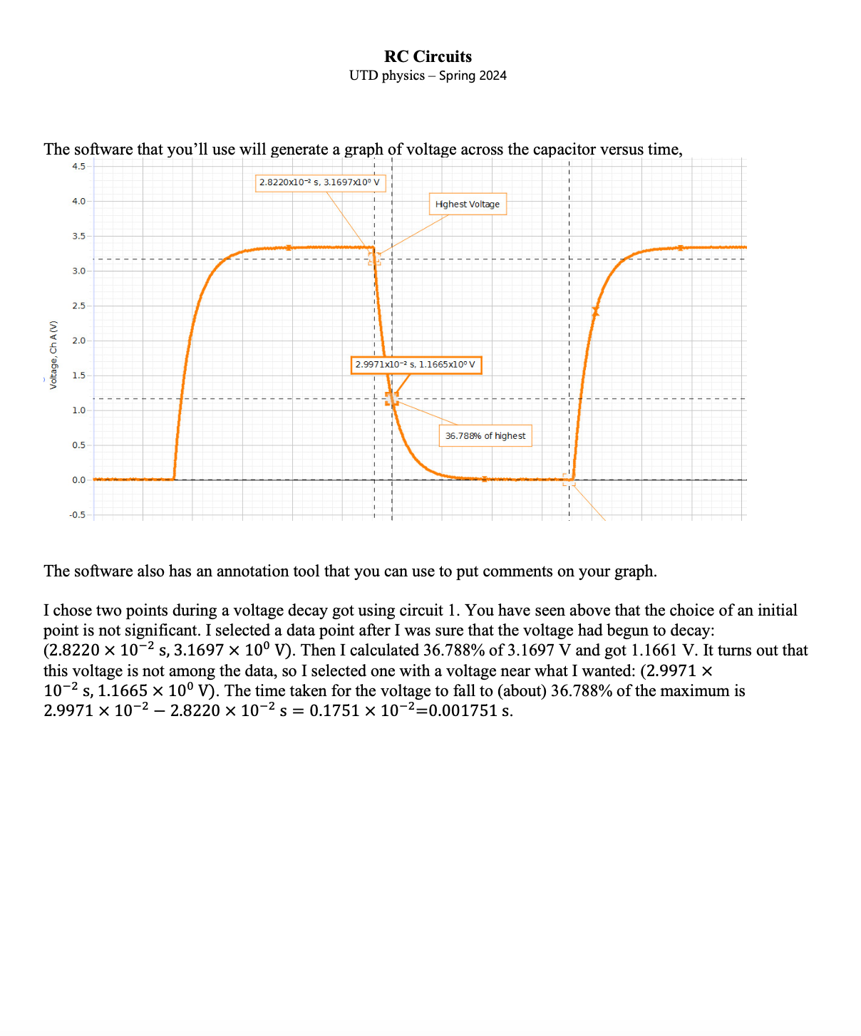
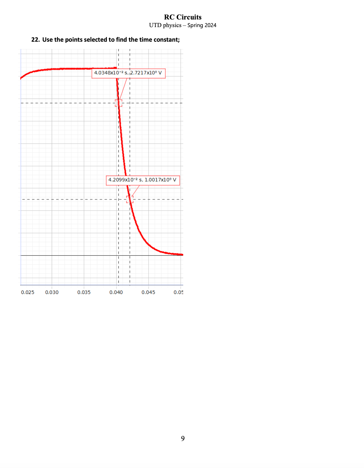
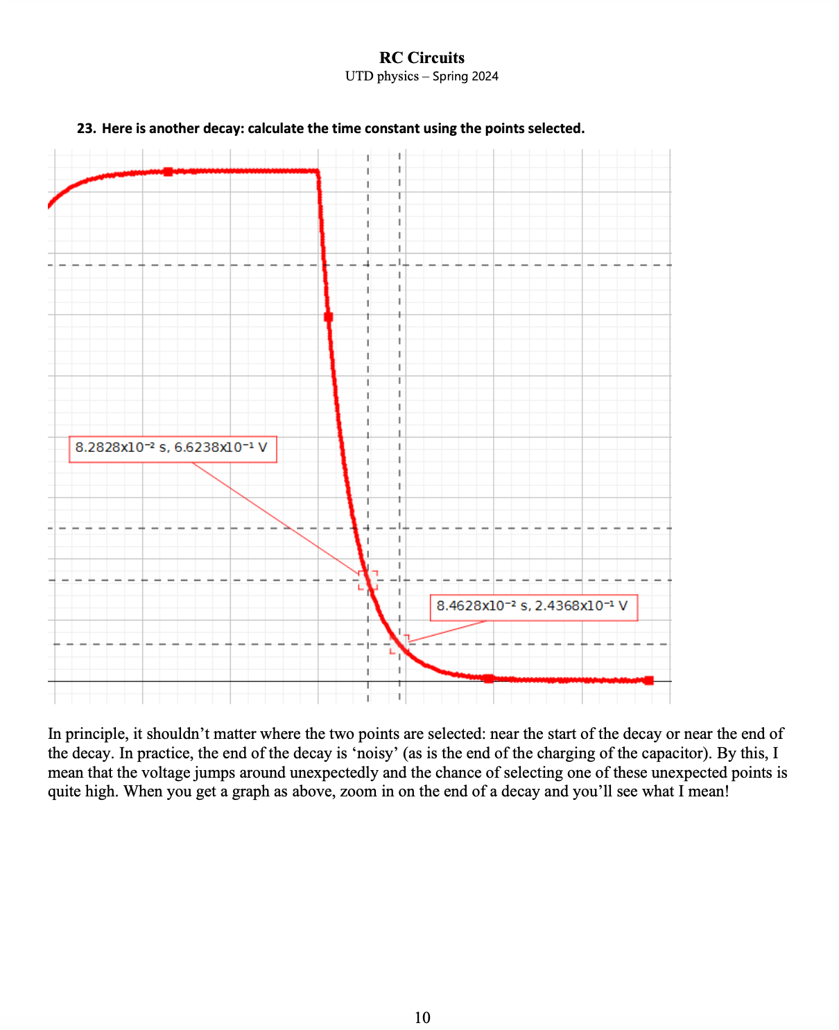
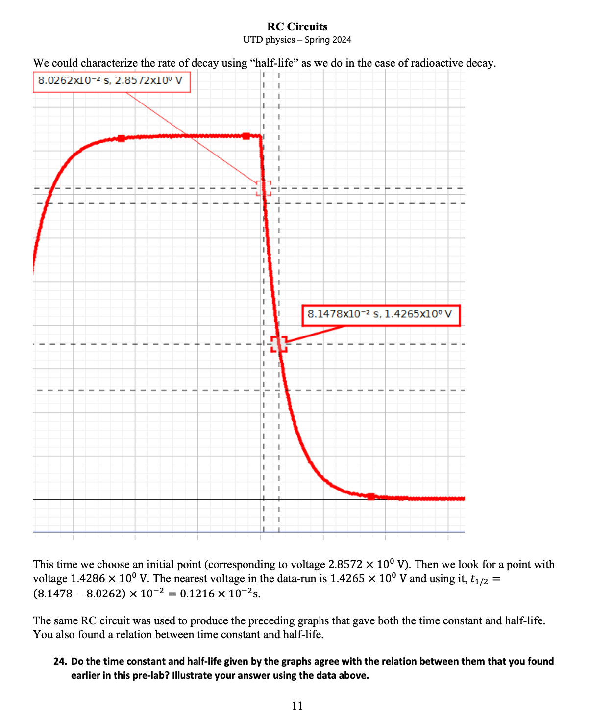
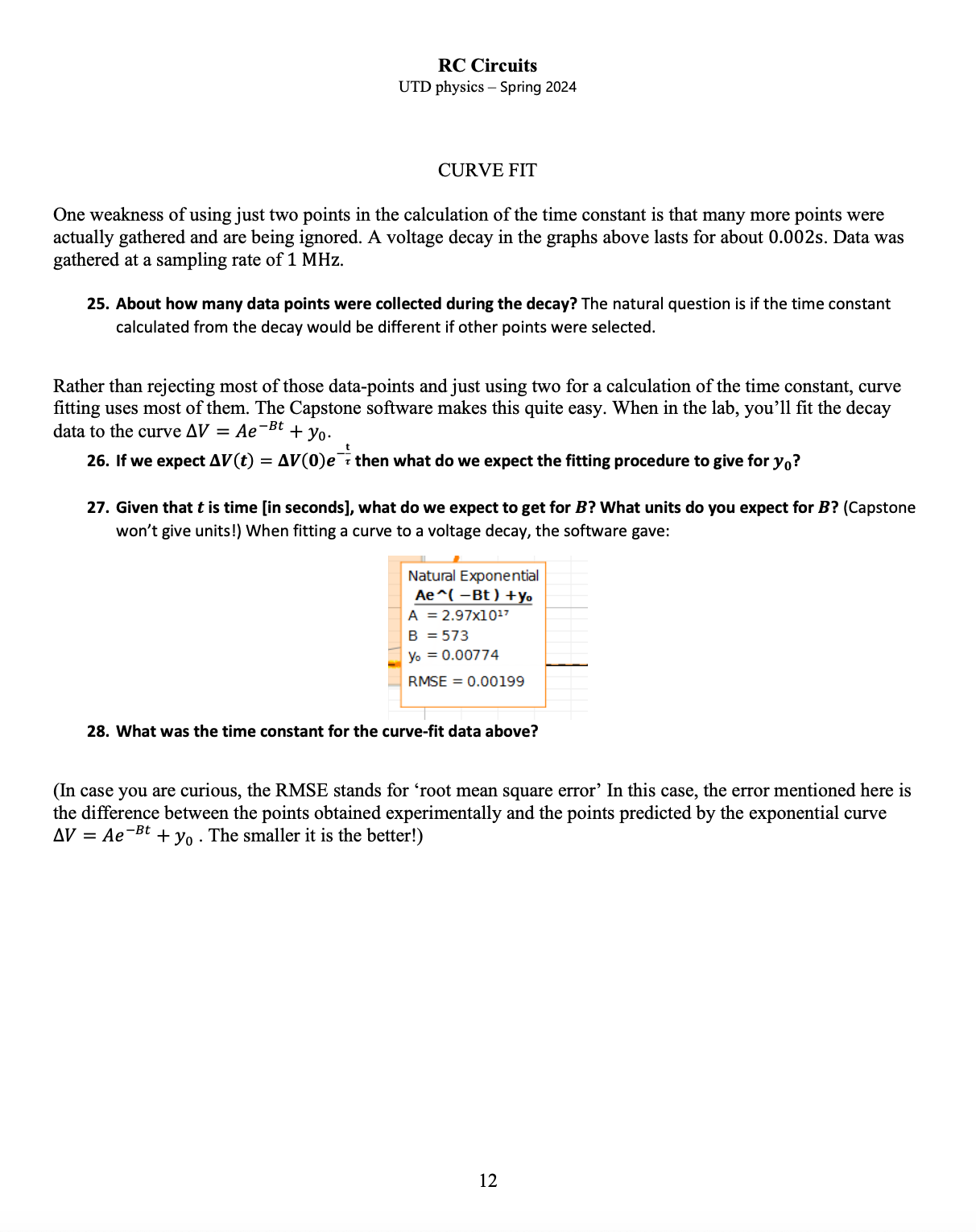
RC Circuits UTD physics Spring 2024 As time approaches any point B, the voltage across the capacitor decays. However, it does not look as if the voltage has 'fully' decayed by the time that the voltage from the signal generator changes at point 5. (The fact that the slope of the capacitor voltage is not zero suggests this.) Remember that this voltage decay is asymptotic so that the slope would decrease a little more if the capacitor was left undisturbed. Similarly, it does not look as if the capacitor has 'fully' charged at any time marked '4' but the signal generator disturbs it before the slope gets near zero. Both the charging and the discharging of the capacitor are asymptotic and will not happen in any finite time. But if we don't disturb the capacitor (by letting the signal generator change voltage), both the charging & discharging will be visibly more complete. In the previous diagram, half the period of the generator (during which a single voltage decay occurs) is about 4t so the period of square waves from the signal generatoris T ~ 87. We'd get a better idea of the voltage being asymptotically approached if we used square waves of a longer period. How long? We want the voltage across Av(e) -t avio) the capacitor to be 'small' enough. Recall 16. What is the ratio of the voltage at t = 20t to the initial voltage across the capacitor? e 1 . . The implication is that we should use a low frequency such as fi,,, = Zor &t which to measure time constants. The circuit that you'll build in the lab is; Circuit 1 R=100kQ C=0.02uF At any moment, there is a difference between the voltage across the signal generator (square wave) and the voltage across the capacitor (exponential increase and decrease). In Electricity V we concluded that \"The sum of pressure differences around a loop that joins one end of the battery to the other is a constant that is a characteristic of the battery\" [This is part of statement 3 c in the model of electricity.] We spoke about pressure differences then, but subsequently replaced this with pofential differences or voltages. Statement 3 c refers to a battery because that was the source of voltage in Electricity V. The signal generator now plays the role of the battery in circuit 1. Statement 3 c tells us that the sum of voltages in circuit 1 is a constant (that is characteristic of the signal generator). In the context of circuit 1, the sum of voltages (that is being supplied by the signal generator) can't change between points A and B [where the sum is zero] or between B and A [where the sum is Vo # 0]. RC Circuits UTD physics Spring 2024 4.5 2.8220x102 s, 3.1697x107 4.0 Hghest Voltage mmmm ko= The software that you'll use will generate a graph 9f voltage across the capacitor versus time, Voltage, Ch A (V) 36.788% of highest The software also has an annotation tool that you can use to put comments on your graph. I chose two points during a voltage decay got using circuit 1. You have seen above that the choice of an initial point is not significant. I selected a data point after I was sure that the voltage had begun to decay: (2.8220 x 1072 5,3.1697 X 10 V). Then I calculated 36.788% of 3.1697 V and got 1.1661 V. It turns out that this voltage is not among the data, so I selected one with a voltage near what I wanted: (2.9971 X 1072 5,1.1665 x 10 V). The time taken for the voltage to fall to (about) 36.788% of the maximum is 29971 x 1072 2.8220 X 1072 s = 0.1751 X 1072=0.001751 s. RC Circuits UTD physics - Spring 2024 22. Use the points selected to find the time constant; 4.0348x10-2 5, 2.7217x10. V 4.2099x10-2 5, 1.0017x100 V 0.025 0.030 0.035 0.040 0.045 0.0 9RC Circuits UTD physics Spring 2024 23. Here is another decay: calculate the time constant using the points selected. 8.2828x1072 5, 6.6238x107* V | ~ I I I I I I I I I I I I t I I I I I I I I I I I I I I I I I I I I I I I I In principle, it shouldn't matter where the two points are selected: near the start of the decay or near the end of the decay. In practice, the end of the decay is 'noisy' (as is the end of the charging of the capacitor). By this, I mean that the voltage jumps around unexpectedly and the chance of selecting one of these unexpected points is quite high. When you get a graph as above, zoom in on the end of a decay and you'll see what I mean! 10 RC Circuits UTD physics Spring 2024 We could characterize the rate of decay using \"half-life\"\" as we do in the case of radioactive decay. 8.0262x1072 5, 2.8572x10V I I I " I I I I - o e o e e o e e e e e e e = e e - o ames s e o o e e e o e e oam|es o 8.1478x1072 5, 1.4265x10V This time we choose an initial point (corresponding to voltage 2.8572 x 10 V). Then we look for a point with voltage 1.4286 x 10 V. The nearest voltage in the data-run is 1.4265 X 10 V and using it, tiz = (8.1478 8.0262) x 1072 = 0.1216 X 107 2s. The same RC circuit was used to produce the preceding graphs that gave both the time constant and half-life. You also found a relation between time constant and half-life. 24. Do the time constant and half-life given by the graphs agree with the relation between them that you found earlier in this pre-lab? Illustrate your answer using the data above. 11 RC Circuits UTD physics Spring 2024 CURVE FIT One weakness of using just two points in the calculation of the time constant is that many more points were actually gathered and are being ignored. A voltage decay in the graphs above lasts for about 0.002s. Data was gathered at a sampling rate of 1 MHz. 25. About how many data points were collected during the decay? The natural question is if the time constant calculated from the decay would be different if other points were selected. Rather than rejecting most of those data-points and just using two for a calculation of the time constant, curve fitting uses most of them. The Capstone software makes this quite easy. When in the lab, you'll fit the decay data to the curve AV = Ae Bt + y,. t 26. If we expect AV(t) = AV(0)e - then what do we expect the fitting procedure to give for y,? 27. Given that t is time [in seconds], what do we expect to get for B? What units do you expect for B? (Capstone won't give units!) When fitting a curve to a voltage decay, the software gave: Natural Exponential Ae~( Bt) +Yo A =2.97x10%7 B =573 o Yo =0.00774 RMSE = 0.00199 28. What was the time constant for the curve-fit data above? (In case you are curious, the RMSE stands for 'root mean square error' In this case, the error mentioned here is the difference between the points obtained experimentally and the points predicted by the exponential curve AV = Ae Bt +y, . The smaller it is the better!) 12