

Referring to Exhibit 3.3 from scenario, then answer the following questions. Phase 1 Identify and diagnose...
Fantastic news! We've Found the answer you've been seeking!
Question:

Transcribed Image Text:
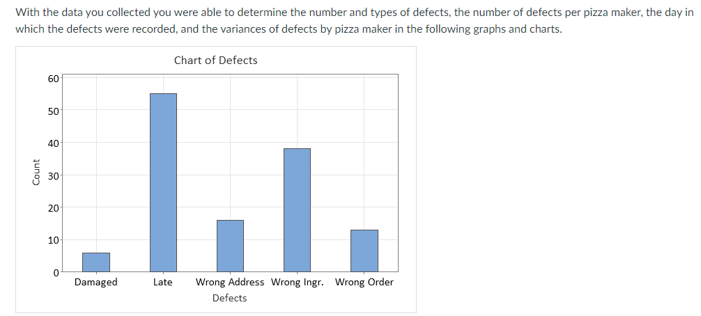
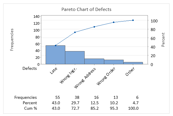
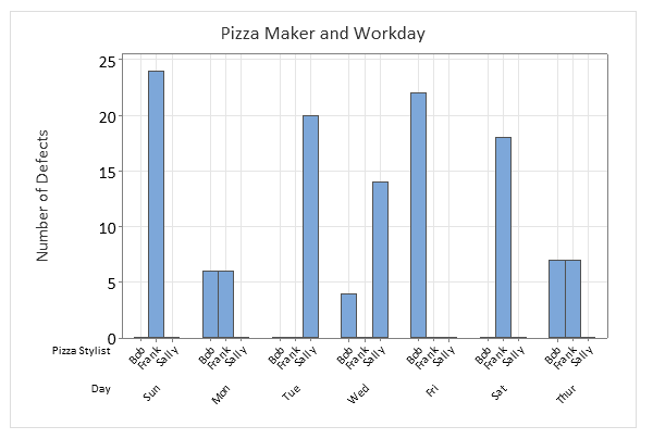
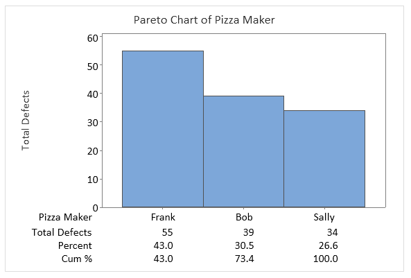
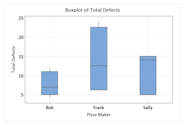
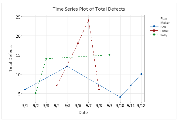
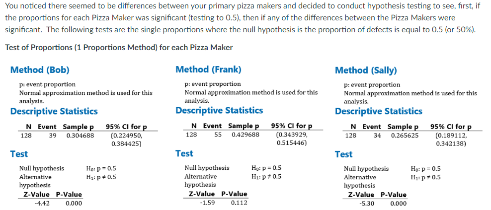
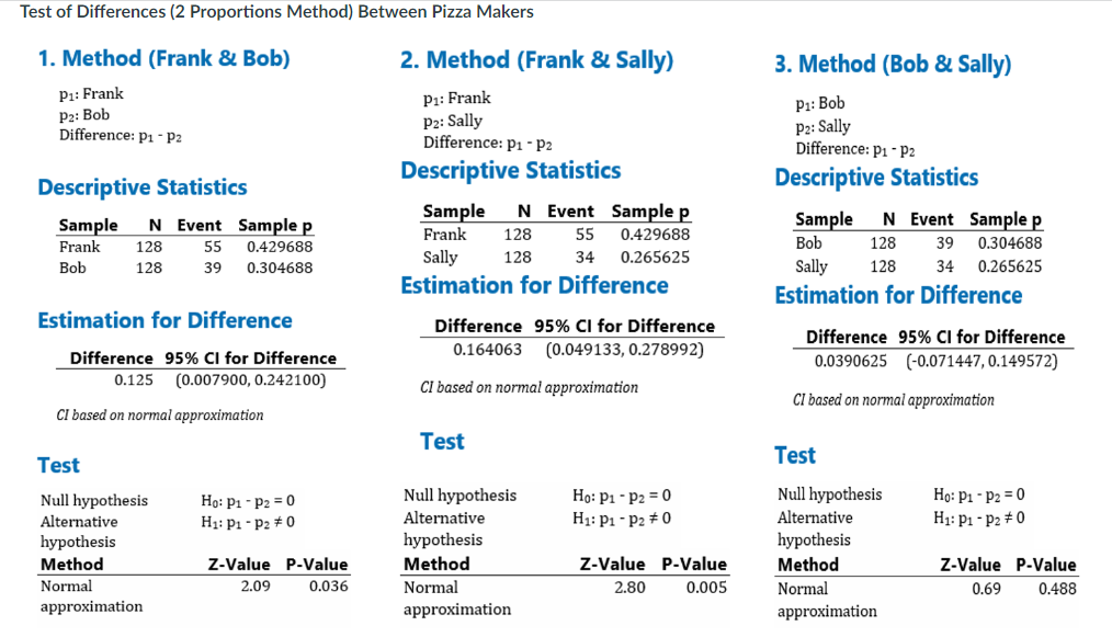
Referring to Exhibit 3.3 from scenario, then answer the following questions. Phase 1 Identify and diagnose the problem Phase 2 Generate alternative solutions , and using the statistics knowledge gained in Modules 1-3, read the given Phase 3 Evaluate alternatives Phase 4 Make the choice Phase 5 Implement the decision Phase 6 Evaluate the decision EXHIBIT 3.3 The Phases of Decision Making Scenario: You are now an assistant manager at Aces & Eights Pizza Company. The store owner was interested in customer service problems with pizzas that were delivered and asked you to find out what was going wrong and to provide your recommendations to improve the overall service. Therefore, over a 12-day period, you recorded how many pizzas were delivered and how many had defects that fell into the following categories: Late, Wrong Ingredients, Wrong Order, Wrong Address, and Damaged. In addition, you recorded the "Pizza Maker" who was making the pizzas each day. You have three primary pizza makers (Bob, Frank, and Sally). Bob had been working for Aces & Eights for a little over a year, Frank had been working for almost two months, and Sally, for about six months. In becoming a Pizza Maker, employees are first trained by the assistant manager for about a week, then they make pizzas under the observation of the "senior Pizza Maker" for approximately two weeks. After which, they are on their own to make pizzas, as the orders come in. With the data you collected you were able to determine the number and types of defects, the number of defects per pizza maker, the day in which the defects were recorded, and the variances of defects by pizza maker in the following graphs and charts. Count 60 50 40 30 20 10 Damaged Chart of Defects 1. Late Wrong Address Wrong Ingr. Wrong Order Defects Frequencie 140 120 100 80 60 40 20 Defects Frequencies Percent Cum % 0 Late 55 43.0 43.0 Pareto Chart of Defects Wrong Ingr. Wrong Address 38 29.7 72.7 16 12.5 85.2 Wrong Order 13 10.2 95.3 Other 6 4.7 100.0 100 80 60 40 20 0 Percent of Defects Number 25 20 15 10 5 0 Pizza Stylist Day Bob Frank Sally Sun Pizza Maker and Workday Bob Frank Sally Mon Bob Frank Sally Tue Bob Frank Sally Wed Bob Frank Sally Fri Bob Frank Sally Sat Bob Frank Sally Thur Total Defects 60 50 40 30 20- 10- 0 Pizza Maker Total Defects Percent Cum % Pareto Chart of Pizza Maker Frank 55 43.0 43.0 Bob 39 30.5 73.4 Sally 34 26.6 100.0 Total Defects 25 20 15 10 5 Bob Boxplot of Total Defects Frank Pizza Maker Sally Total Defects 25 20 15 10 5 Time Series Plot of Total Defects 9/1 9/2 9/3 9/4 9/5 9/6 9/7 9/8 9/9 9/10 9/11 9/12 Date Pizza Maker Bob Frank Sally You noticed there seemed to be differences between your primary pizza makers and decided to conduct hypothesis testing to see, first, if the proportions for each Pizza Maker was significant (testing to 0.5), then if any of the differences between the Pizza Makers were significant. The following tests are the single proportions where the null hypothesis is the proportion of defects is equal to 0.5 (or 50%). Test of Proportions (1 Proportions Method) for each Pizza Maker Method (Bob) p: event proportion Normal approximation method is used for this analysis. Descriptive Statistics N Event Sample p 39 128 0.304688 Test Null hypothesis Alternative hypothesis Z-Value P-Value -4.42 0.000 95% CI for p (0.224950, 0.384425) Ho: p = 0.5 H: p = 0.5 Method (Frank) p: event proportion Normal approximation method is used for this analysis. Descriptive Statistics N Event Sample p 128 55 0.429688 Test Null hypothesis Alternative hypothesis Z-Value P-Value -1.59 0.112 95% CI for p (0.343929, 0.515446) Ho: p = 0.5 H: p = 0.5 Method (Sally) p: event proportion Normal approximation method is used for this analysis. Descriptive Statistics N Event Sample p 34 128 0.265625 Test Null hypothesis Alternative hypothesis Z-Value P-Value -5.30 0.000 95% CI for p (0.189112, 0.342138) Ho: p = 0.5 H: p * 0.5 Test of Differences (2 Proportions Method) Between Pizza Makers 1. Method (Frank & Bob) P: Frank P2: Bob Difference: P-P2 Descriptive Statistics Sample N Event Sample p Frank 128 Bob 128 55 0.429688 39 0.304688 Estimation for Difference Difference 95% CI for Difference 0.125 (0.007900, 0.242100) CI based on normal approximation Test Null hypothesis Alternative hypothesis Method Normal approximation Ho: P1-P2 = 0 H: P1 P2 0 Z-Value P-Value 2.09 0.036 2. Method (Frank & Sally) P: Frank P2: Sally Difference: P P2 Descriptive Statistics Sample N Event Sample p Frank 128 55 0.429688 Sally 128 34 0.265625 Estimation for Difference Difference 95% CI for Difference 0.164063 (0.049133, 0.278992) CI based on normal approximation Test Null hypothesis Alternative hypothesis Method Normal approximation Ho: P1 - P2 = 0 H: P1 - P2 #0 Z-Value P-Value 2.80 0.005 3. Method (Bob & Sally) P: Bob P2: Sally Difference: P1-P2 Descriptive Statistics Sample N Event Sample p Bob 128 39 0.304688 Sally 128 34 0.265625 Estimation for Difference Difference 95% CI for Difference 0.0390625 (-0.071447, 0.149572) CI based on normal approximation Test Null hypothesis Alternative hypothesis Method Normal approximation Ho: P1 P2 = 0 H: P1 P2 0 Z-Value P-Value 0.69 0.488 Questions: 1. Fully describe the problem or opportunity in this scenario. 2. Fully develop and describe at least two alternatives (DO NOT analyze the alternatives here). 3. Fully analyze each alternative. 4. Provide your recommended alternative and provide the details as to why it is the best alternative. Referring to Exhibit 3.3 from scenario, then answer the following questions. Phase 1 Identify and diagnose the problem Phase 2 Generate alternative solutions , and using the statistics knowledge gained in Modules 1-3, read the given Phase 3 Evaluate alternatives Phase 4 Make the choice Phase 5 Implement the decision Phase 6 Evaluate the decision EXHIBIT 3.3 The Phases of Decision Making Scenario: You are now an assistant manager at Aces & Eights Pizza Company. The store owner was interested in customer service problems with pizzas that were delivered and asked you to find out what was going wrong and to provide your recommendations to improve the overall service. Therefore, over a 12-day period, you recorded how many pizzas were delivered and how many had defects that fell into the following categories: Late, Wrong Ingredients, Wrong Order, Wrong Address, and Damaged. In addition, you recorded the "Pizza Maker" who was making the pizzas each day. You have three primary pizza makers (Bob, Frank, and Sally). Bob had been working for Aces & Eights for a little over a year, Frank had been working for almost two months, and Sally, for about six months. In becoming a Pizza Maker, employees are first trained by the assistant manager for about a week, then they make pizzas under the observation of the "senior Pizza Maker" for approximately two weeks. After which, they are on their own to make pizzas, as the orders come in. With the data you collected you were able to determine the number and types of defects, the number of defects per pizza maker, the day in which the defects were recorded, and the variances of defects by pizza maker in the following graphs and charts. Count 60 50 40 30 20 10 Damaged Chart of Defects 1. Late Wrong Address Wrong Ingr. Wrong Order Defects Frequencie 140 120 100 80 60 40 20 Defects Frequencies Percent Cum % 0 Late 55 43.0 43.0 Pareto Chart of Defects Wrong Ingr. Wrong Address 38 29.7 72.7 16 12.5 85.2 Wrong Order 13 10.2 95.3 Other 6 4.7 100.0 100 80 60 40 20 0 Percent of Defects Number 25 20 15 10 5 0 Pizza Stylist Day Bob Frank Sally Sun Pizza Maker and Workday Bob Frank Sally Mon Bob Frank Sally Tue Bob Frank Sally Wed Bob Frank Sally Fri Bob Frank Sally Sat Bob Frank Sally Thur Total Defects 60 50 40 30 20- 10- 0 Pizza Maker Total Defects Percent Cum % Pareto Chart of Pizza Maker Frank 55 43.0 43.0 Bob 39 30.5 73.4 Sally 34 26.6 100.0 Total Defects 25 20 15 10 5 Bob Boxplot of Total Defects Frank Pizza Maker Sally Total Defects 25 20 15 10 5 Time Series Plot of Total Defects 9/1 9/2 9/3 9/4 9/5 9/6 9/7 9/8 9/9 9/10 9/11 9/12 Date Pizza Maker Bob Frank Sally You noticed there seemed to be differences between your primary pizza makers and decided to conduct hypothesis testing to see, first, if the proportions for each Pizza Maker was significant (testing to 0.5), then if any of the differences between the Pizza Makers were significant. The following tests are the single proportions where the null hypothesis is the proportion of defects is equal to 0.5 (or 50%). Test of Proportions (1 Proportions Method) for each Pizza Maker Method (Bob) p: event proportion Normal approximation method is used for this analysis. Descriptive Statistics N Event Sample p 39 128 0.304688 Test Null hypothesis Alternative hypothesis Z-Value P-Value -4.42 0.000 95% CI for p (0.224950, 0.384425) Ho: p = 0.5 H: p = 0.5 Method (Frank) p: event proportion Normal approximation method is used for this analysis. Descriptive Statistics N Event Sample p 128 55 0.429688 Test Null hypothesis Alternative hypothesis Z-Value P-Value -1.59 0.112 95% CI for p (0.343929, 0.515446) Ho: p = 0.5 H: p = 0.5 Method (Sally) p: event proportion Normal approximation method is used for this analysis. Descriptive Statistics N Event Sample p 34 128 0.265625 Test Null hypothesis Alternative hypothesis Z-Value P-Value -5.30 0.000 95% CI for p (0.189112, 0.342138) Ho: p = 0.5 H: p * 0.5 Test of Differences (2 Proportions Method) Between Pizza Makers 1. Method (Frank & Bob) P: Frank P2: Bob Difference: P-P2 Descriptive Statistics Sample N Event Sample p Frank 128 Bob 128 55 0.429688 39 0.304688 Estimation for Difference Difference 95% CI for Difference 0.125 (0.007900, 0.242100) CI based on normal approximation Test Null hypothesis Alternative hypothesis Method Normal approximation Ho: P1-P2 = 0 H: P1 P2 0 Z-Value P-Value 2.09 0.036 2. Method (Frank & Sally) P: Frank P2: Sally Difference: P P2 Descriptive Statistics Sample N Event Sample p Frank 128 55 0.429688 Sally 128 34 0.265625 Estimation for Difference Difference 95% CI for Difference 0.164063 (0.049133, 0.278992) CI based on normal approximation Test Null hypothesis Alternative hypothesis Method Normal approximation Ho: P1 - P2 = 0 H: P1 - P2 #0 Z-Value P-Value 2.80 0.005 3. Method (Bob & Sally) P: Bob P2: Sally Difference: P1-P2 Descriptive Statistics Sample N Event Sample p Bob 128 39 0.304688 Sally 128 34 0.265625 Estimation for Difference Difference 95% CI for Difference 0.0390625 (-0.071447, 0.149572) CI based on normal approximation Test Null hypothesis Alternative hypothesis Method Normal approximation Ho: P1 P2 = 0 H: P1 P2 0 Z-Value P-Value 0.69 0.488 Questions: 1. Fully describe the problem or opportunity in this scenario. 2. Fully develop and describe at least two alternatives (DO NOT analyze the alternatives here). 3. Fully analyze each alternative. 4. Provide your recommended alternative and provide the details as to why it is the best alternative.
Expert Answer:

Related Book For 
Applied Regression Analysis and Other Multivariable Methods
ISBN: 978-1285051086
5th edition
Authors: David G. Kleinbaum, Lawrence L. Kupper, Azhar Nizam, Eli S. Rosenberg
Posted Date:
Students also viewed these finance questions
-
Planning is one of the most important management functions in any business. A front office managers first step in planning should involve determine the departments goals. Planning also includes...
-
Read the article "An Unholy Trinity: Three Ways Employees Embezzle Cash." Describe how billing schemes, payroll schemes, and expense reimbursement schemes are perpetrated to answer the following...
-
Episode 1: A New War Begines Vanderbilt How did Vanderbilts upbringing affect his business attitudes? Which product Vanderbilt decided to sell, as he knew good entrepreneur find something that...
-
Explain what CVA and DVA measure?
-
In 2009, Simplon Merchandising, Inc., sold its interest in a chain of wholesale outlets, taking the company completely out of the wholesaling business. The company still operates its retail outlets....
-
You are in an elevator moving between two floors of a building at constant speed. Compare the work done on you by the elevator when you are moving upward to a higher floor to the work done when you...
-
What is the within-sector selection effect for each individual sector? Primo Management Co. is looking at how best to evaluate the performance of its managers. Primo has been hearing more and more...
-
19. Find the tension T for the system shown in figure :- T T T 1 kg 2 kg 3 kg (1) IgN (2) 2 gN (3) 5 gN (4) 6 gN 20. A ball of mass 0.5 kg moving with a velocity of 2 m/sec strikes a wall normally...
-
Suppose that the interest rate on a one-year Treasury bill is currently 6% and that investors expect that the interest rates on one-year Treasury bills over the next three years will be 7%, 8%, and...
-
The information on earnings and deductions for the pay period ended December 14 from King Company's payroll records is as follows: Beginning Cumulative Name Gross Pay Earnings Burgess, J. L. $410...
-
How do theories of motivation apply to the design of incentive systems in a sales-driven corporate environment? Explain
-
How do theories of work-life balance apply to the development of policies in organizations that operate across different cultural contexts? Explain
-
You would like to give your child $100,000 to start a career 25 years from now. How much money must you set aside today for this purpose if you can earn 7.0 percent on your investments?
-
In a diverse workplace, explain how the concepts of cultural awareness, cultural safety, and cultural competence impact the following work roles: HR Manager in a diverse center Educator of the...
-
If Susanna Metro invests 7,009.87 now and she will receive 20,000 at the end of 11 years, what annual rate of interest will she be earning on her investment? Future value of 1Factor 7%, 11 years...
-
For the vector whose polar components are (Vr = 1, Vθ = 0), compute in polars all components of the second covariant derivative Vα;μ;ν. To find...
-
Examine the five pairs of data points given in the following table. a. What is the mathematical relationship between X and Y? b. Show by computation that, for the straight-line regression of Y on X,...
-
This time including SEX as a predictor (coded SEX = 1 if female, SEX = 0 if male). a. Examine a plot of the studentized or jackknife residuals versus the predicted values. Are any regression...
-
The data listed in the following table are from a study by Benignus and others (1981). Blood and brain levels of toluene (a commonly used solvent) were measured in rats following a 3-hour inhalation...
-
Consider an EPR state \(|\phiangle_{A B}\); Alice measures the spin on \(z\), then Bob measures it on \(x\), and then Alice measures it again on \(z\). Classify the possible answers for the second...
-
Explore whether the original Bell inequality can be violated at large angles as well.
-
Instead of the Bell-CHSH inequality in the text, consider an inequality obtained in the same way from \(\tilde{M}=\left(A+A^{\prime} ight) B^{\prime}+\left(A-A^{\prime} ight) B\) instead of \(M\). Is...

Study smarter with the SolutionInn App