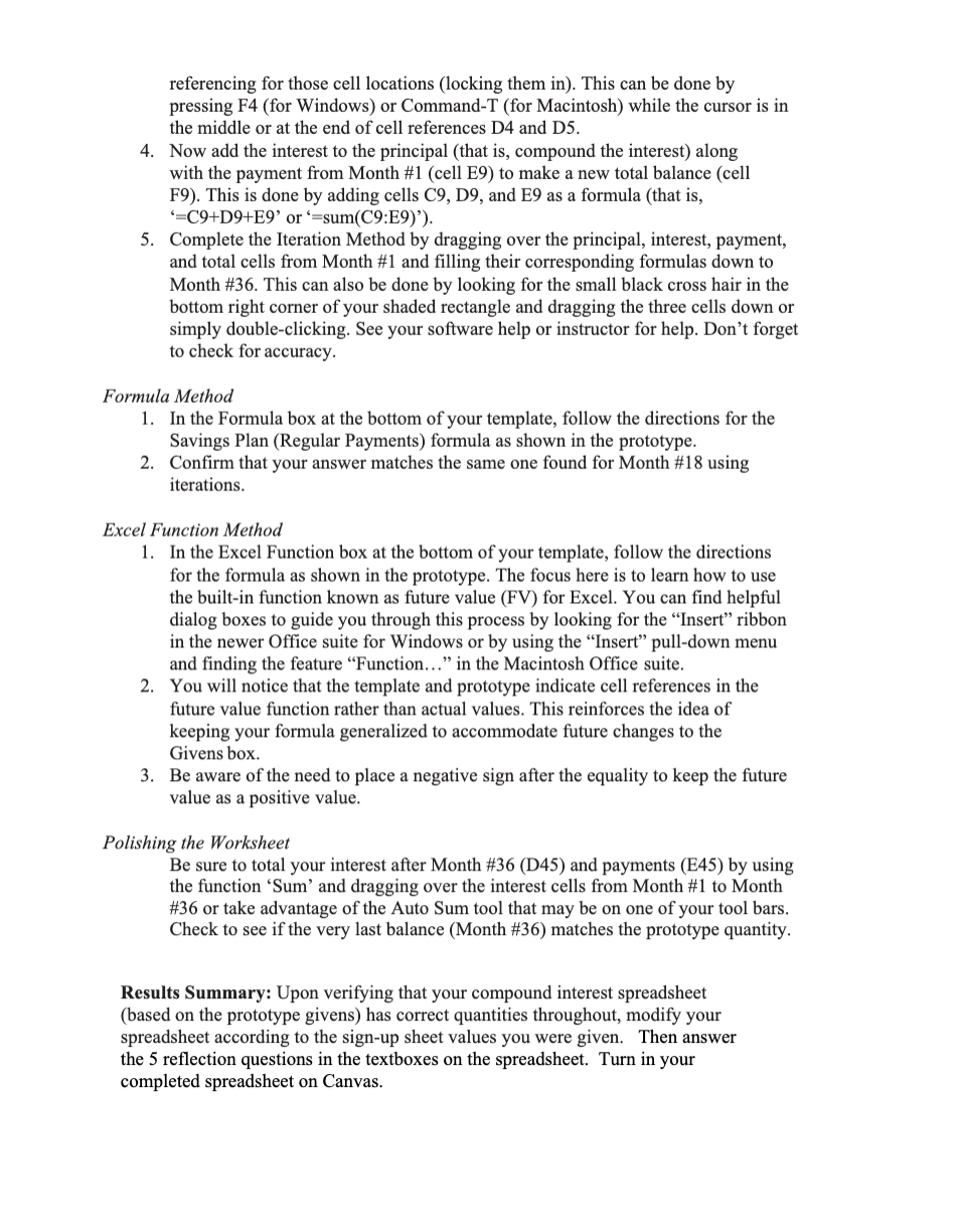
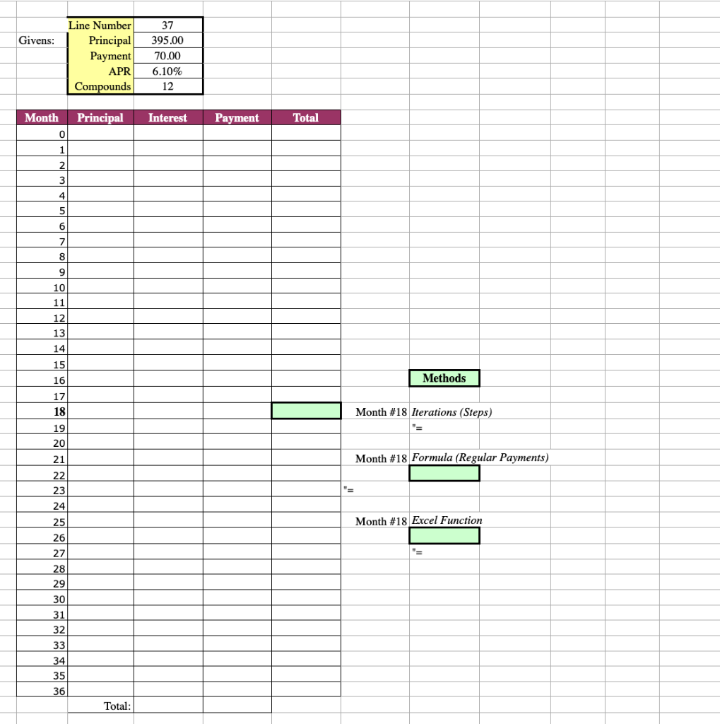
Regular Payments Savings Plan A Three Methods Approach Before you begin: Look for your name on the sign-up sheet (given by your instructor) and copy the Line #, Principal, and APR. Review the savings plan formula (regular payments) from section 4-C of your text. Remember that all formulas in an Excel spreadsheet begin with an equality symbol'='. Recall that to reference a cell, you can click on it or type its column letter and row number. Download Spreadsheet: Download or ask your instructor for the file "Savings_Plan_Template.xls" which provides you a spreadsheet framework. This helps you concentrate on the three methods of calculating the lump sum investment without worrying about the formatting details. Procedure: Using the template you have downloaded and the prototype figure below, construct a savings plan spreadsheet using three different methods iteration (steps), formula, and Excel function) that will arrive at the very same balance if properly done. Be sure to type in the Givens box the same principal, compound, and APR as the prototype figure. From Month #18 (row 26) and thereafter, you will be building formulas that are flexible enough to accommodate other values you type into the Givens box later. hard M IWPRTO Manhatonal Foll 4 11 VO 15 SMS PRINT 01 1980 1 SM 21 25 TIK A1914 11 4331 100 29 Iterations (Steps) Method 1. Link by a cell reference, the total cell of Month #0 (cell F8) to the principal in the Givens box (cell D2). 2. Now let principal from Month #1 (cell C9) reference from the total (cell F8). 3. For the interest in Month #1 (cell D9), create a formula by multiplying the principal (cell C9) by the given APR (cell D4) divided by the given Compounds (cell D5). Note: because you will want to always use the same given APR and compound values even after you copy or fill the formulas down the columns, you must use absolute cell 2001 249.14 7 NE DD 78231 K 13 15 895. 912.50 4231 CON 11 15 301 Machinery 2013 1102 . 944 103 10510 10 HO 21 22 23 20 une Mosch Must L.1.12 14137. ISSN 0045 18.000 1144 Mach19 26 29 128.00 118 al 451 42 47 481 40 14100 123231 IS IN 15201 1151 250 2900 18 IK 2300 DS 130 VI 1941 1000 1 21 30 1191 141.21 14122 15 592 141 13. 12 WHO 37 Givens: Line Number Principal Payment APR Compounds 395.00 70.00 6.10% 12 Month Principal Interest Payment Total 0 1 2 3 4 5 6 7 8 9 10 11 12 13 14 15 16 Methods Month #18 Iterations (Steps) 17 18 19 20 21 Month #18 Formula (Regular Payments) 22 23 24 Month #18 Excel Function 25 26 "= 27 28 29 30 31 32 33 34 35 36 Total: Regular Payments Savings Plan A Three Methods Approach Before you begin: Look for your name on the sign-up sheet (given by your instructor) and copy the Line #, Principal, and APR. Review the savings plan formula (regular payments) from section 4-C of your text. Remember that all formulas in an Excel spreadsheet begin with an equality symbol'='. Recall that to reference a cell, you can click on it or type its column letter and row number. Download Spreadsheet: Download or ask your instructor for the file "Savings_Plan_Template.xls" which provides you a spreadsheet framework. This helps you concentrate on the three methods of calculating the lump sum investment without worrying about the formatting details. Procedure: Using the template you have downloaded and the prototype figure below, construct a savings plan spreadsheet using three different methods iteration (steps), formula, and Excel function) that will arrive at the very same balance if properly done. Be sure to type in the Givens box the same principal, compound, and APR as the prototype figure. From Month #18 (row 26) and thereafter, you will be building formulas that are flexible enough to accommodate other values you type into the Givens box later. hard M IWPRTO Manhatonal Foll 4 11 VO 15 SMS PRINT 01 1980 1 SM 21 25 TIK A1914 11 4331 100 29 Iterations (Steps) Method 1. Link by a cell reference, the total cell of Month #0 (cell F8) to the principal in the Givens box (cell D2). 2. Now let principal from Month #1 (cell C9) reference from the total (cell F8). 3. For the interest in Month #1 (cell D9), create a formula by multiplying the principal (cell C9) by the given APR (cell D4) divided by the given Compounds (cell D5). Note: because you will want to always use the same given APR and compound values even after you copy or fill the formulas down the columns, you must use absolute cell 2001 249.14 7 NE DD 78231 K 13 15 895. 912.50 4231 CON 11 15 301 Machinery 2013 1102 . 944 103 10510 10 HO 21 22 23 20 une Mosch Must L.1.12 14137. ISSN 0045 18.000 1144 Mach19 26 29 128.00 118 al 451 42 47 481 40 14100 123231 IS IN 15201 1151 250 2900 18 IK 2300 DS 130 VI 1941 1000 1 21 30 1191 141.21 14122 15 592 141 13. 12 WHO 37 Givens: Line Number Principal Payment APR Compounds 395.00 70.00 6.10% 12 Month Principal Interest Payment Total 0 1 2 3 4 5 6 7 8 9 10 11 12 13 14 15 16 Methods Month #18 Iterations (Steps) 17 18 19 20 21 Month #18 Formula (Regular Payments) 22 23 24 Month #18 Excel Function 25 26 "= 27 28 29 30 31 32 33 34 35 36 Total