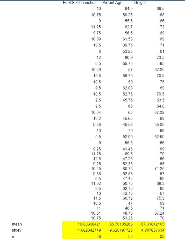
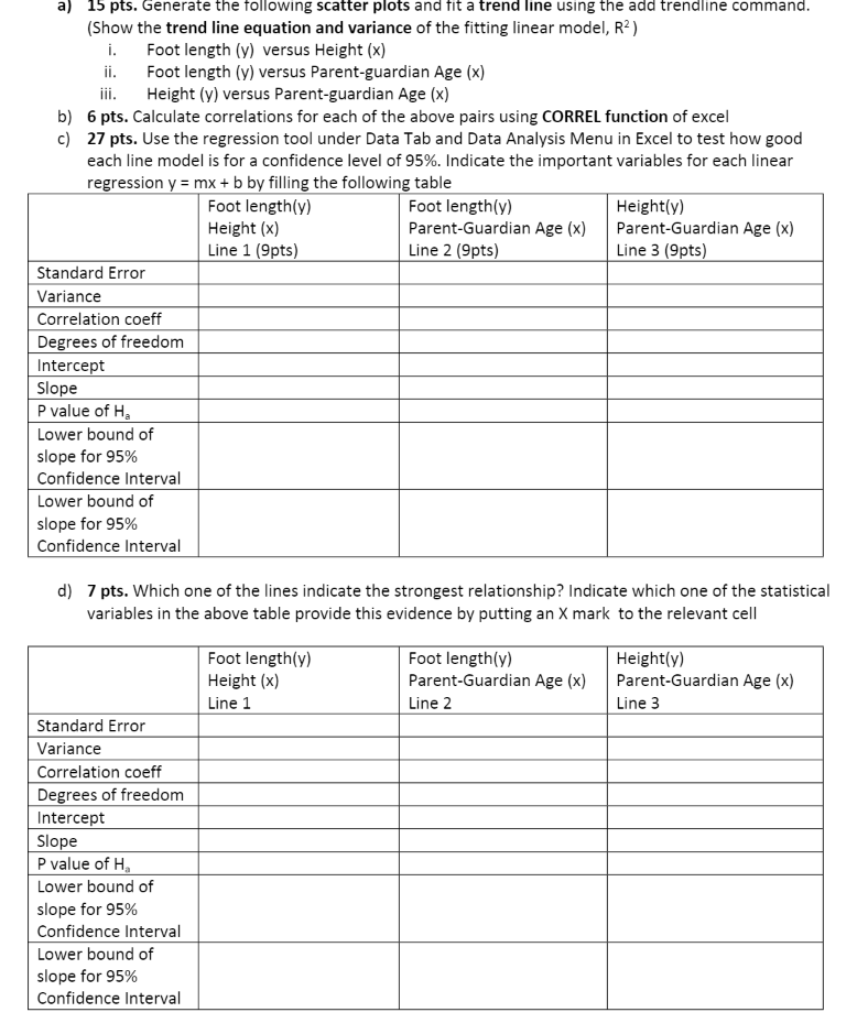
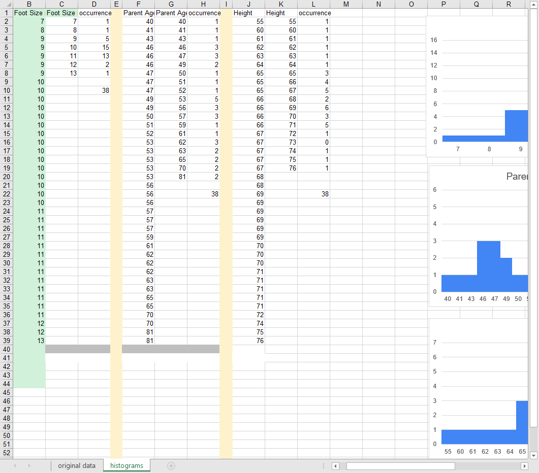
s.Convert the given histograms to a cumulative distribution function by dividing each bar with n, sample size. Draw the cumulative distribution functions (Hint: Area under the curve is equal to 1 in the cumulative distribution function. But the area under the curve in these histograms is equal to n. This is why we need to divide by n) Estimate by using the cumulative distribution functions above: A. What is the probability for the student to have a height of higher than 69 inches B. What is the probability for the student to have a foot length between 11-12 inches (including 11,12) C. What is the probability for the student to have a parent/legal guardian of age less than 57 3. Transfer the above measurements (69, 11-12, 57) to z scores and fill the table below: Mean () Std Dev (0) Actual value 69 11,12 Height Foot length Parent-guardian Age 57 Z score s. Assuming your data was distributed normally, repeat the estimations in question 2, this time using Z table (Use NORM.s.DIST function of excel or your calculator or the z table in class slides) A. What is the probability for the student to have a height of higher than 69 inches B. What is the probability for the student to have a foot length between 11-12 inches (including 11,12) C. What is the probability for the student to have a parent/legal guardian of age less than 57 ! ... Comment for each one of your random variables separately: Is the probability almost the same when you use the z table versus your own histogram? Why or why not? A) Height variable: B) Foot length variable: C) Parent-legal guardian Age variable: mean stdev n Foot Size in inches 10 10.75 9 11.25 9.75 10.09 10.5 8 12 9.5 10.56 10.5 10.5 9.5 10.5 9.5 9.5 10.04 10.2 9.38 10 9.5 9 9.25 11.25 12.5 9.25 10.25 9.88 6.5 11.02 9.5 10 11.5 10.5 11 10.51 10.75 Parent Age 38 64.5 59.25 55.5 62.7 56.5 61.58 39.75 53.25 80.9 55.75 57 56.75 50 62.08 52.75 45.75 65 62 45.65 45.58 70 52.99 55.5 41.45 69.5 47.25 52.33 80.75 52.58 47.45 50.75 62.75 42.75 60.75 47 48.6 48.75 53.25 10.08368421 55.70105263 1.062842749 9.620197725 38 Height 69.5 68 66 72 69 69 71 61 73.5 65 67.25 70.5 75 69 70.5 63.5 64.8 67.32 68 55.35 66 62.99 66 69 70 66 65 71.25 67 62 69.3 60 67 75.5 69 71 67.24 70 67.61842105 4.047637634 38 a) 15 pts. Generate the following scatter plots and fit a trend line using the add trendline command. (Show the trend line equation and variance of the fitting linear model, R) i. ii. Foot length (y) versus Height (x) Foot length (y) versus Parent-guardian Age (x) iii. Height (y) versus Parent-guardian Age (x) b) 6 pts. Calculate correlations for each of the above pairs using CORREL function of excel c) 27 pts. Use the regression tool under Data Tab and Data Analysis Menu in Excel to test how good each line model is for a confidence level of 95%. Indicate the important variables for each linear regression y = mx + b by filling the following table Standard Error Variance Correlation coeff Degrees of freedom Intercept Slope P value of H Lower bound of slope for 95% Confidence Interval Lower bound of slope for 95% Confidence Interval Standard Error Variance Correlation coeff Degrees of freedom Intercept d) 7 pts. Which one of the lines indicate the strongest relationship? Indicate which one of the statistical variables in the above table provide this evidence by putting an X mark to the relevant cell Slope P value of H Lower bound of slope for 95% Foot length(y) Height (x) Line 1 (9pts) Confidence Interval Lower bound of slope for 95% Confidence Interval Foot length(y) Parent-Guardian Age (x) Line 2 (9pts) Foot length(y) Height (x) Line 1 Height(y) Parent-Guardian Age (x) Line 3 (9pts) Foot length(y) Parent-Guardian Age (x) Line 2 Height(y) Parent-Guardian Age (x) Line 3 B D 1 Foot Size Foot Size occurrence 2 7 3 4 5 6 7 8 9 10 11 12 13 14 15 16 17 18 19 20 21 22 23 24 25 26 27 28 29 30 31 32 33 34 35 36 37 38 39 40 41 42 43 44 45 46 47 48 49 50 51 52 7 8 9 9 9 9 9 10 10 10 10 10 10 10 10 10 10 10 10 10 10 10 11 11 11 11 11 11 11 11 11 11 11 11 11 12 12 13 068 9 10 11 12 13 original data 1 1 5 15 13 2 1 38 E F G H Parent Age Parent Age occurrence 40 40 histograms 41 43 46 46 46 47 47 47 49 49 50 51 52 53 53 53 53 53 56 56 56 57 57 57 59 61 62 62 62 63 63 65 65 70 70 81 81 + 41 43 46 47 49 50 51 52 53 56 57 59 61 62 63 65 70 81 1 1 1 3 3 2 1 1 1 5 3 3 1 1 3 2 2 2 2 38 I J Height 55 60 61 62 63 64 65 65 65 66 66 66 66 67 67 67 67 67 88888888RRRFFENNEG 68 68 69 69 69 69 69 69 70 70 70 71 71 71 71 71 72 74 75 76 K Height 55 60 61 62 63 64 65 66 1488N NEG C3STOTI 67 68 69 70 71 72 73 74 75 occurrence 76 1 1 1 1 1 1 3 4 5 2 6 5 1 0 1 1 1 38 M N O 16 24 20 14 12 10 8 6 4 2 0 6 5 4 3 2 1 0 7 6 5 4 3 2 1 0 P 7 Q 8 R 9 Parel 40 41 43 46 47 49 50 55 60 61 62 63 64 65