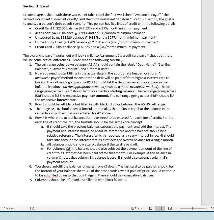
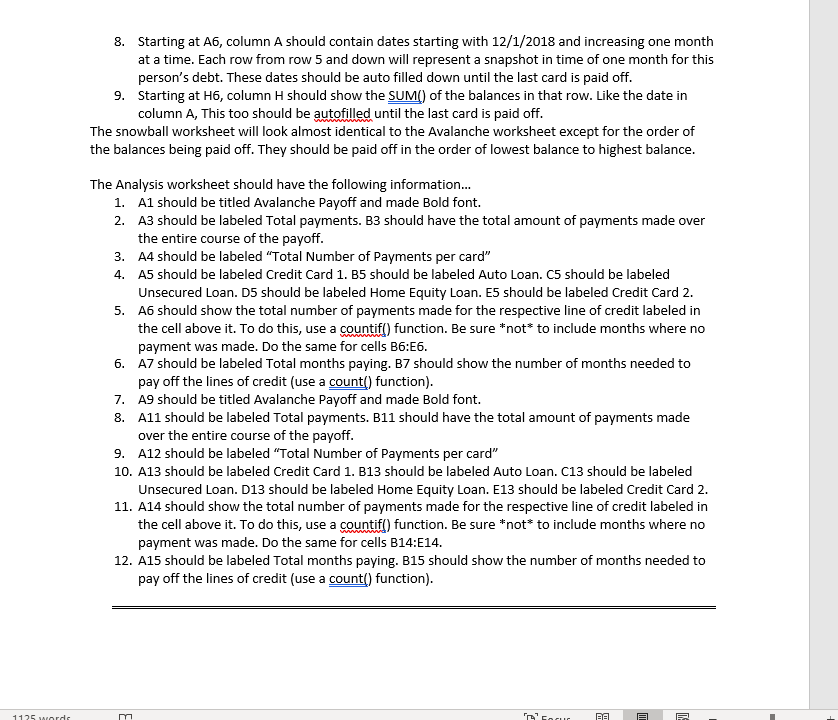
Section 1: Excel Create a spreadsheet with three worksheet tabs. Label the first worksheet "Avalanche Payoff," the second worksheet "Snowball Payoff," and the third worksheet "Analysis." For this question, the goal is to analyze a person's debt payoff scenario. This person has five lines of credit with the following details: Credit Card 1: $2100 balance @ 8.99% and a $75/month minimum payment Auto Loan: $4800 balance @ 2.99% and a $135/month minimum payment Unsecured Loan: $13520 balance @ 9.99% and a $277/month minimum payment Home Equity Loan: $21709 balance @ 2.75% and a $325/month minimum payment Credit Card 2: $850 balance @ 6.99% and a $40/month minimum payment The avalanche payoff worksheet will look similar to Assignment 2's credit card payoff sheet but there will be some critical differences. Please read the following carefully... 1. The cell range going down between A1:A4 should contain the labels "Debt Name", "Starting Balance", "Payment Amount", and "Interest Rate" 2. Now you need to start filling in the actual data in the appropriate header locations. An avalanche payoff method means that the debt will be paid off from highest interest rate to lowest. The cell range going across B1:F1 should list the debt names as they appear in the bulleted list above (in the appropriate order as prescribed in the avalanche method). The cell range going across B2:F2 should list the respective starting balance. The cell range going across B3:F3 should list the respective payment amount. The cell range going across B4:F4 should list the respective interest rate. 3. Row 5 should be left blank but filled in with black fill color between the A5:45 cell range. 4. The range B6:F6, should have a formula that makes that balance equal to the balance in the respective row 2 cell that you entered for #2 above. 5. Row 7 is where the actual balance formulas need to be entered for each line of credit. For the each line of credit column, the formula should be the same core concept... a. It should take the previous balance, subtract the payment, and add the interest. The payment and interest should be absolute references and the balance should be a relative reference. The interest (which is reported as a yearly interest in row 4) should take into account the interest rate as it reflects the overall balance for a single month. b. All balances should show a zero balance if the card is paid off. c. For columns C:F, the balance should also subtract the payment amount of the line of credit to its left that has been paid off for that month. For example, if the balance in column C notes that column B's balance is zero, it should also subtract column B's payment amount. 6. You should autofill the balance formulas from #5 down. The last card to be paid off should be the bottom of your balance sheet. All of the other cards (even if paid off prior) should continue to be autofilled down to that point. Again, there should be no negative balances. 7. Column G should be left blank but filled in with black fill color. 1125 words D Focus @ -- + 10 8. Starting at A6, column A should contain dates starting with 12/1/2018 and increasing one month at a time. Each row from row 5 and down will represent a snapshot in time of one month for this person's debt. These dates should be auto filled down until the last card is paid off. 9. Starting at H6, column H should show the SUM) of the balances in that row. Like the date in column A, This too should be autofilled until the last card is paid off. The snowball worksheet will look almost identical to the Avalanche worksheet except for the order of the balances being paid off. They should be paid off in the order of lowest balance to highest balance. The Analysis worksheet should have the following information... 1. Al should be titled Avalanche Payoff and made Bold font. 2. A3 should be labeled Total payments. B3 should have the total amount of payments made over the entire course of the payoff. 3. A4 should be labeled "Total Number of Payments per card" 4. AS should be labeled Credit Card 1. B5 should be labeled Auto Loan. CS should be labeled Unsecured Loan. D5 should be labeled Home Equity Loan. E5 should be labeled Credit Card 2. 5. A6 should show the total number of payments made for the respective line of credit labeled in the cell above it. To do this, use a countif() function. Be sure *not* to include months where no payment was made. Do the same for cells B6:56. 6. A7 should be labeled Total months paying. B7 should show the number of months needed to pay off the lines of credit (use a count() function). 7. A9 should be titled Avalanche Payoff and made Bold font. 8. A11 should be labeled Total payments. B11 should have the total amount of payments made over the entire course of the payoff. 9. A12 should be labeled "Total Number of Payments per card" 10. A13 should be labeled Credit Card 1. B13 should be labeled Auto Loan. C13 should be labeled Unsecured Loan. D13 should be labeled Home Equity Loan. E13 should be labeled Credit Card 2. 11. A14 should show the total number of payments made for the respective line of credit labeled in the cell above it. To do this, use a countif() function. Be sure *not* to include months where no payment was made. Do the same for cells B14:E14. 12. A15 should be labeled Total months paying. B15 should show the number of months needed to pay off the lines of credit (use a count() function). 1125 ordem Scorur PE Section 1: Excel Create a spreadsheet with three worksheet tabs. Label the first worksheet "Avalanche Payoff," the second worksheet "Snowball Payoff," and the third worksheet "Analysis." For this question, the goal is to analyze a person's debt payoff scenario. This person has five lines of credit with the following details: Credit Card 1: $2100 balance @ 8.99% and a $75/month minimum payment Auto Loan: $4800 balance @ 2.99% and a $135/month minimum payment Unsecured Loan: $13520 balance @ 9.99% and a $277/month minimum payment Home Equity Loan: $21709 balance @ 2.75% and a $325/month minimum payment Credit Card 2: $850 balance @ 6.99% and a $40/month minimum payment The avalanche payoff worksheet will look similar to Assignment 2's credit card payoff sheet but there will be some critical differences. Please read the following carefully... 1. The cell range going down between A1:A4 should contain the labels "Debt Name", "Starting Balance", "Payment Amount", and "Interest Rate" 2. Now you need to start filling in the actual data in the appropriate header locations. An avalanche payoff method means that the debt will be paid off from highest interest rate to lowest. The cell range going across B1:F1 should list the debt names as they appear in the bulleted list above (in the appropriate order as prescribed in the avalanche method). The cell range going across B2:F2 should list the respective starting balance. The cell range going across B3:F3 should list the respective payment amount. The cell range going across B4:F4 should list the respective interest rate. 3. Row 5 should be left blank but filled in with black fill color between the A5:45 cell range. 4. The range B6:F6, should have a formula that makes that balance equal to the balance in the respective row 2 cell that you entered for #2 above. 5. Row 7 is where the actual balance formulas need to be entered for each line of credit. For the each line of credit column, the formula should be the same core concept... a. It should take the previous balance, subtract the payment, and add the interest. The payment and interest should be absolute references and the balance should be a relative reference. The interest (which is reported as a yearly interest in row 4) should take into account the interest rate as it reflects the overall balance for a single month. b. All balances should show a zero balance if the card is paid off. c. For columns C:F, the balance should also subtract the payment amount of the line of credit to its left that has been paid off for that month. For example, if the balance in column C notes that column B's balance is zero, it should also subtract column B's payment amount. 6. You should autofill the balance formulas from #5 down. The last card to be paid off should be the bottom of your balance sheet. All of the other cards (even if paid off prior) should continue to be autofilled down to that point. Again, there should be no negative balances. 7. Column G should be left blank but filled in with black fill color. 1125 words D Focus @ -- + 10 8. Starting at A6, column A should contain dates starting with 12/1/2018 and increasing one month at a time. Each row from row 5 and down will represent a snapshot in time of one month for this person's debt. These dates should be auto filled down until the last card is paid off. 9. Starting at H6, column H should show the SUM) of the balances in that row. Like the date in column A, This too should be autofilled until the last card is paid off. The snowball worksheet will look almost identical to the Avalanche worksheet except for the order of the balances being paid off. They should be paid off in the order of lowest balance to highest balance. The Analysis worksheet should have the following information... 1. Al should be titled Avalanche Payoff and made Bold font. 2. A3 should be labeled Total payments. B3 should have the total amount of payments made over the entire course of the payoff. 3. A4 should be labeled "Total Number of Payments per card" 4. AS should be labeled Credit Card 1. B5 should be labeled Auto Loan. CS should be labeled Unsecured Loan. D5 should be labeled Home Equity Loan. E5 should be labeled Credit Card 2. 5. A6 should show the total number of payments made for the respective line of credit labeled in the cell above it. To do this, use a countif() function. Be sure *not* to include months where no payment was made. Do the same for cells B6:56. 6. A7 should be labeled Total months paying. B7 should show the number of months needed to pay off the lines of credit (use a count() function). 7. A9 should be titled Avalanche Payoff and made Bold font. 8. A11 should be labeled Total payments. B11 should have the total amount of payments made over the entire course of the payoff. 9. A12 should be labeled "Total Number of Payments per card" 10. A13 should be labeled Credit Card 1. B13 should be labeled Auto Loan. C13 should be labeled Unsecured Loan. D13 should be labeled Home Equity Loan. E13 should be labeled Credit Card 2. 11. A14 should show the total number of payments made for the respective line of credit labeled in the cell above it. To do this, use a countif() function. Be sure *not* to include months where no payment was made. Do the same for cells B14:E14. 12. A15 should be labeled Total months paying. B15 should show the number of months needed to pay off the lines of credit (use a count() function). 1125 ordem Scorur PE