Question: Select an appropriate forecasting method and use the method to forecast the demand for quarters I, II, III, and IV for years 6 to 8.

Select an appropriate forecasting method and use the method to forecast the demand for quarters I, II, III, and IV for years 6 to 8.

PLEASE NOTE: THIS HAS NOTHING TO DO WITH CLEAR OR BLACK PLASTIC!! STOP GIVING ME THOSE ANSWERS.

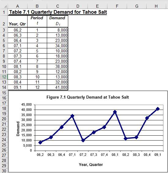
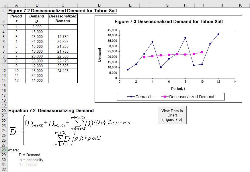
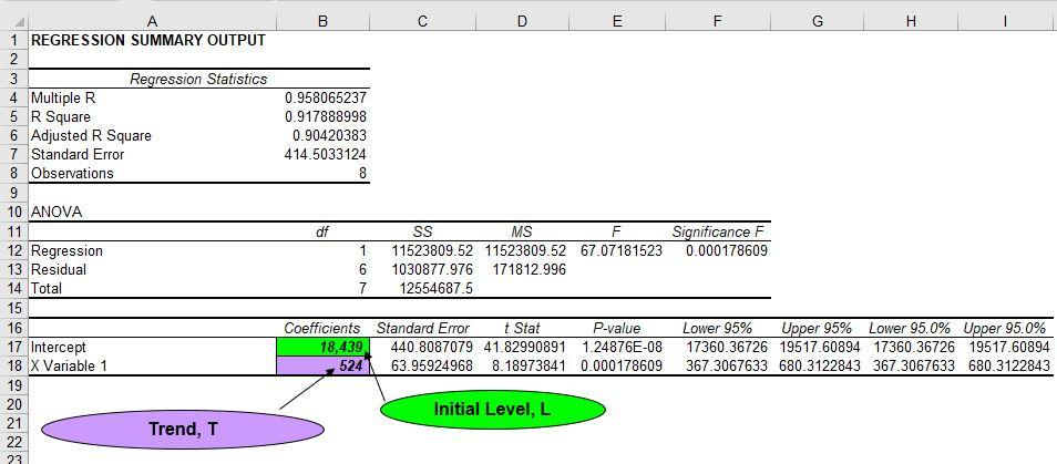
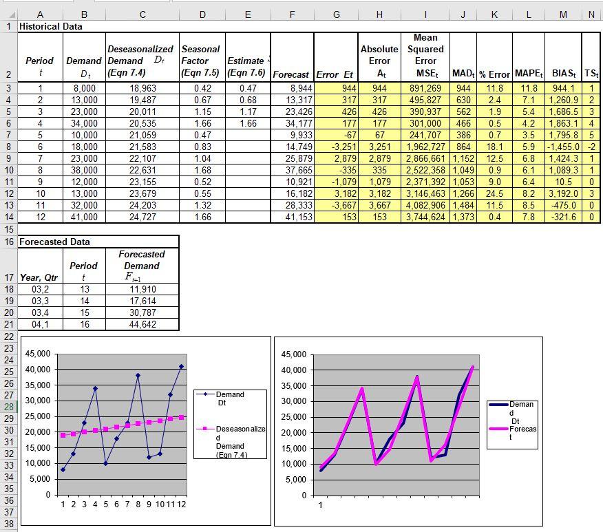
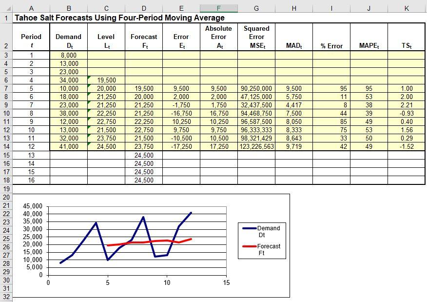
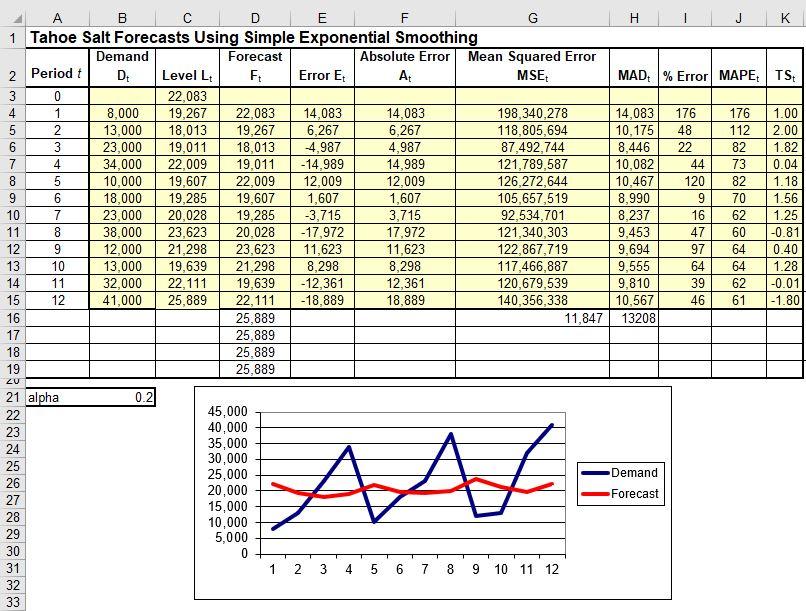
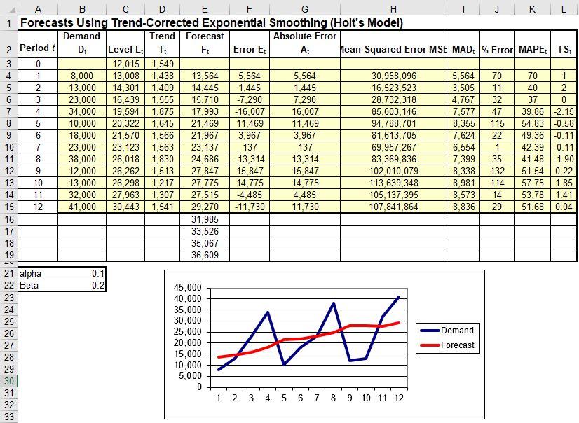
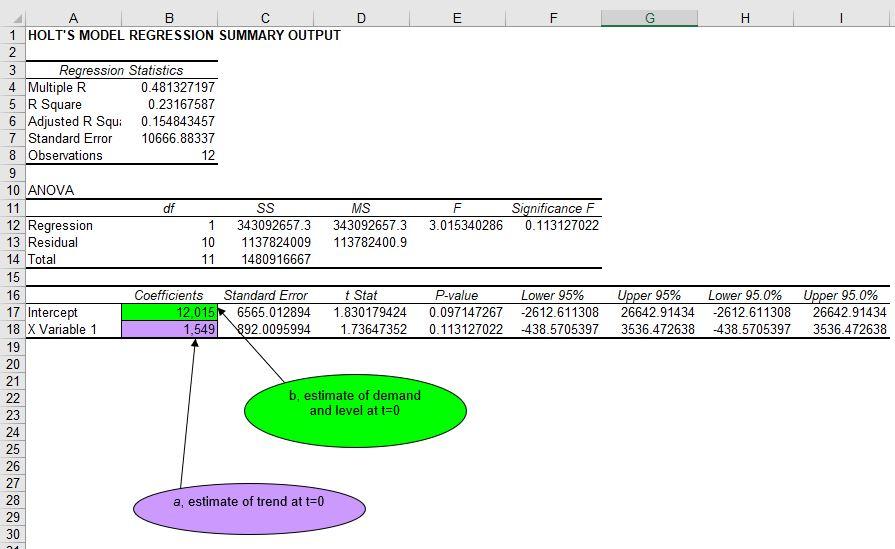
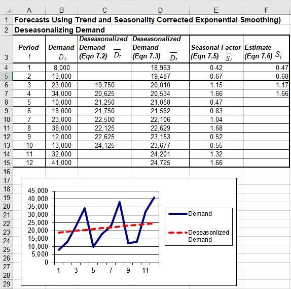
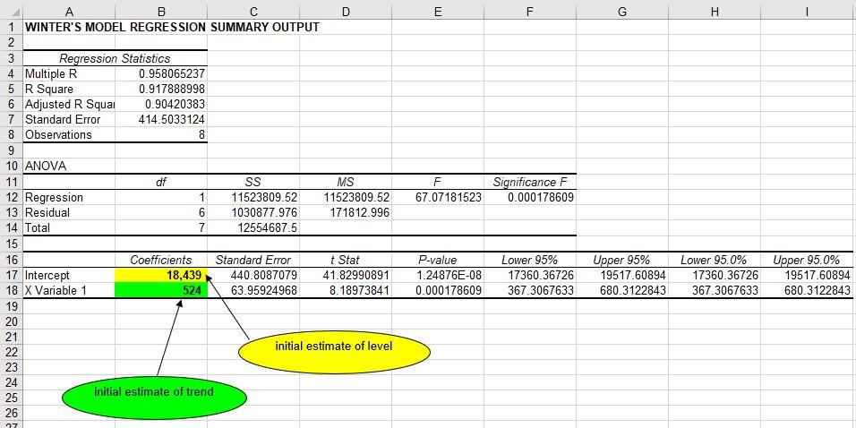
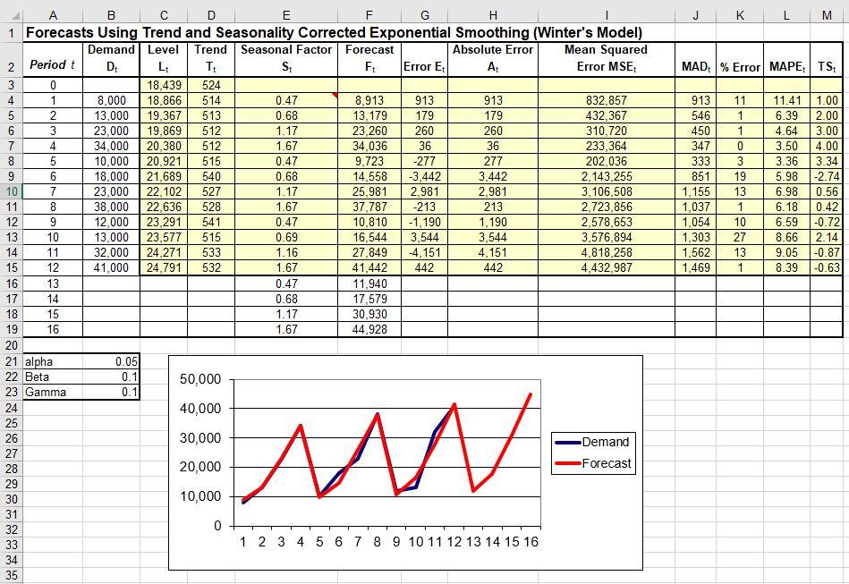
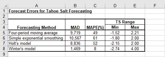
FORECASTING METHODS ARE USED WITHIN THE GIVEN SPREADSHEETS. PLEASE CHOOSE ONE, FOLLOW THE ABOVE DIRECTIONS, AND WRITE A BRIEF EXPLANATION FOR WHY YOU CHOSE THAT METHOD. Select an appropriate forecasting method and use

LL B DE G H 1 Table 7.1 Quarterly Demand for Tahoe Salt Period Demand 2 Year, Qtr t D: 3 06,2 1 8,000 4 06,3 2 13,000 5 06,4 3 23,000 6 07,1 4 34,000 7 07,2 5 10,000 8 07,3 6 18,000 07,4 7 23,000 10 08,1 8 38,000 11 08,2 9 12,000 12 08,3 10 13,000 13 08,4 11 32,000 14 09,1 12 41,000 15 16 Figure 7.1 Quarterly Demand at Tahoe Salt 17 45,000 18 40,000 19 35,000 20 30,000 21 25,000 22 20,000 23 15,000 24 10,000 25 5,000 26 0 27 06,206,3 06,4 07,1 07,207,3 07,4 08,1 08,208,308,409,1 28 29 Year, Quarter 30 Demand A E K Demand ON 0 14 A B D F G H J 1 Figure 7.2 Deseasonalized Demand for Tahoe Salt Period Demand Deseasonalized 2 t D Demand Figure 7.3 Deseasonalized Demand for Tahoe Salt 3 1 8,000 4 2 13,000 45,000 3 23,000 19,750 40,000 6 4 34,000 20,625 35,000 7 5 10,000 21,250 30,000 8 6 18,000 21,750 25,000 9 7 23,000 22,500 20,000 10 8 38,000 22, 125 15,000 11 9 12,000 22,625 10,000 12 10 13,000 24 125 5,000 13 11 32,000 0 14 12 41,000 2 6 8 10 12 15 16 Period, t 17 -Demand... Deseasonalized Demand 18 19 20 Equation 7.2 Deseasonalizing Demand View Data in 21 7-14p/2) Chart 22 (Figure 7.3) 23 i=+-(p/2) /2] 25 26 27 i=1p/2] 28 where: 29 D = Demand 30 p = periodicity 31 t = period 32 24 D. {D:-p2) + Datpi2+ 2D}/{2p} forpeven ED. p for podd B D E F G H 1 REGRESSION SUMMARY OUTPUT 2 3 Regression Statistics 4 Multiple R 5 R Square 6 Adjusted R Square 7 Standard Error 8 Observations 9 10 ANOVA 11 12 Regression 13 Residual 14 Total 0.958065237 0.917888998 0.90420383 414.5033124 8 df Significance F 0.000178609 1 6 7 SS MS F 11523809.52 11523809.52 67.07181523 1030877.976 171812.996 12554687.5 Coefficients Standard Error t Stat P-value 18,439 440.8087079 41.82990891 1.24876E-08 524 63.95924968 8.18973841 0.000178609 Lower 95% Upper 95% Lower 95.0% Upper 95.0% 17360.36726 19517.60894 17360.36726 19517.60894 367.3067633 680.3122843 367.3067633 680.3122843 16 17 Intercept 18 X Variable 1 19 20 21 22 23 Initial Level, L Trend, T Olo wol D E G H J KL M N 1 Historical Data Mean Deseasonalized Seasonal Absolute Squared Period Demand Demand D: Factor Estimate Error Error 2 t D (Egn 7.4) (Eqn 7.5) (Eqn 7.6) Forecast Error Et At MSE MAD% Error MAPE BIASt TS 3 1 8,000 18,963 0.42 0.47 8,944 944 944 891,269 944 11.8 11.8 944.1 1 4 2 13,000 19,487 0.67 0.68 13,317 317 317 495,827 630 2.4 7.1 1,260.9 2 5 3 23,000 20,011 1.15 1.17 23,426 426 426 390,937 562 1.9 5.4 1,686.5 3 4 34,000 20,535 1.66 1.66 34,177 177 177 301,000 466 0.5 4.2 1,863.1 4 5 10,000 21,059 0.47 9.933 -67 67 241,707 386 0.7 3.5 1,795.8 5 8 6 18,000 21,583 0.83 14,7491 -3,251 3,251 1,962,727 864 18.1 5.9 -1,455.0 -2 7 23,000 22, 107 1.04 25,879 2,879 2,879 2,866,661 1,152 12.5 6.8 1,424.3 1 10 8 38,000 22,631 1.68 37,665 -335 335 2,522,358 1,049 0.9 6.1 1,089.3 1 11 9 12,000 23,155 0.52 10,921 -1,079 1,079 2,371,392 1,053 9.0 6.4 10.5 0 12 10 13,000 23,679 0.55 16,182 3,182 3,182 3,146,463 1,266 24.5 8.2 3,192.0 3 13 11 32,000 24,203 1.32 28,333 -3,667 3,667 4,082,906 1,484 11.5 8.5 -475.0 14 12 41,000 24,727 1.66 41,153 153 153 3,744,624 1,373 0.4 7.8 -321.6 15 16 Forecasted Data Forecasted Period Demand 17 Year, Qtr t F 18 03,2 13 11,910 19 14 17,614 20 03,4 30,787 21 04,1 44,642 22 23 45,000 45,000 24 25 40,000 40,000 2635,000 35,000 27 Demand 30,000 Dt 28 30,000 Deman 25,000 d Dt 3020,000 Deseason alize 20,000 Forecas d t 31 32 15,000 Demand 15,000 (Egn 7.4) 3310,000 10,000 34 5,000 5,000 35 0 0 36 1 2 3 4 5 6 7 8 9 10 11 12 1 37 38 -1 16. 29 25,000 G H K Squared Error MSE MADE % Error MAPE TSE 00 90,250,000 47,125,000 32,437,500 94,468,750 96,587,500 96,333,333 98,321,429 123,226,563 9,500 5,750 4,417 7,500 8,050 8,333 8,643 9,719 95 11 8 44 85 75 33 42 95 53 38 39 49 53 50 49 1.00 2.00 2.21 -0.93 0.40 1.56 0.29 -1.52 A B D E 1 Tahoe Salt Forecasts Using Four-Period Moving Average Absolute Period Demand Level Forecast Error Error 2 t Dt Lt Ft Et At 3 1 8,000 4 2 13,000 5 3 23,000 6 4 34,000 19,500 10,000 20,000 19,500 9,500 9,500 8 18,000 21,250 20,000 2,000 2,000 9 7 23,000 21,250 21,250 -1,750 1,750 10 8 38,000 22,250 21,250 -16,750 16,750 11 9 12,000 22,750 22,250 10,250 10,250 12 10 13,000 21,500 22,750 9,750 9,750 13 11 32,000 23,750 21,500 - 10,500 10,500 14 12 41,000 24,500 23,750 -17,250 17,250 15 13 24,500 16 14 24,500 17 15 24,500 18 16 24,500 19 20 21 45,000 22 40,000 23 35,000 24 30,000 25 25,000 26 20,000 27 15,000 28 10,000 5,000 29 0 30 0 5 10 15 31 32 Demand Dt M - Forecast Ft 00 H K MAD % Error MAPETS A B D E F G 1 Tahoe Salt Forecasts Using Simple Exponential Smoothing Demand Forecast Absolute Error Mean Squared Error 2 Period DI Level Lt Ft Error E At MSE 3 0 22,083 4 1 8,000 19,267 22,083 14,083 14,083 198,340,278 5 2 13,000 18,013 19,267 6,267 6,267 118,805,694 6 3 23,000 19.011 18,013 4,987 4,987 87,492,744 4 34,000 22,009 19.011 - 14,989 14,989 121,789,587 8 5 10,000 19,607 22,009 12,009 12,009 126,272,644 9 6 18,000 19,285 19,607 1,607 1,607 105,657,519 10 7 23,000 20,028 19,285 3,715 3,715 92,534,701 11 8 38,000 23,623 20.028 -17,972 17,972 121,340,303 12 9 12,000 21,298 23,623 11,623 11,623 122,867,719 13 10 13,000 19,639 21,298 8,298 8,298 117,466,887 14 11 32,000 22,111 19,639 -12,361 12,361 120,679,539 15 12 41,000 25,889 22,111 -18.889 18,889 140,356,338 16 25,889 11,847 17 25,889 18 25,889 19 25,889 14,083 10,175 8,446 10,082 10,467 8,990 8,237 9,453 9,694 9,555 9,810 10,567 13208 176 48 22 44 120 9 16 47 97 64 39 46 176 112 82 73 82 70 62 60 64 64 62 61 1.00 2.00 1.82 0.04 1.18 1.56 1.25 -0.81 0.40 1.28 -0.01 -1.80 ZU 0.2 21 alpha 22 23 24 25 26 27 28 29 30 31 32 33 45,000 40,000 35,000 30,000 25,000 20,000 15,000 10,000 5,000 0 X -Demand Forecast 1 2 3 4 5 6 7 8 9 10 11 12 ON N A B C D E F G H J K L 1 Forecasts Using Trend-Corrected Exponential Smoothing (Holt's Model) Demand Trend Forecast Absolute Error 2 Period D Level LTE Ft Error Et At Mean Squared Error MSE MAD % Error MAPE TS 3 0 12,015 1,549 4 1 8,000 13,008 1,438 13,564 5,564 5,564 30,958,096 5,564 70 70 1 5 2 13,000 14,301 1,409 14,445 1,445 1.445 16,523,523 3,505 11 40 2 6 3 23,000 16,439 1,555 15,710 -7,290 7,290 28,732,318 4,767 32 37 7 4 34,000 19,594 1,875 17,993 -16,007 16,007 85,603, 146 7,577 47 39.86 -2.15 5 10,000 20,322 1,645 21,469 11,469 11,469 94,788,701 8,355 115 54.83 -0.58 9 6 18,000 21,570 1,566 21,967 3,967 3,967 81,613,705 7,624 22 49.36 -0.11 10 7 23,000 23,123 1,563 23,137 137 137 69,957,267 6,554 1 42.39 -0.11 11 8 38,000 26,018 1,830 24,686 -13,314 13,314 83,369,836 7,399 35 41.48 -1.90 12 9 12,000 26,262 1,513 27,847 15,847 15,847 102,010,079 8,338 132 51.54 0.22 13 10 13,000 26,298 1,217 27,775 14,775 14,775 113,639,348 8,981 114 57.75 1.85 14 11 32,000 27,963 1,307 27,515 4,485 4,485 105,137,395 8,573 14 53.78 1.41 15 12 41,000 30,443 1,541 29,270 -11,730 11,730 107,841,864 8,836 29 51.68 0.04 16 31,985 17 33,526 18 35,067 19 36,609 21 alpha 0.1 22 Beta 0.2 45,000 23 40,000 24 35,000 25 30,000 26 25,000 -Demand 27 20,000 -Forecast 28 15,000 29 10,000 5,000 30 0 31 1 2 3 4 5 6 7 8 9 10 11 12 32 33 CON 20 AN f D ITI F G H 1 SS F 3.015340286 Significance F 0.113127022 A B 1 HOLT'S MODEL REGRESSION SUMMARY OUTPUT 2 3 Regression Statistics 4 Multiple R 0.481327197 5 R Square 0.23167587 6 Adjusted R Squi 0.154843457 7 Standard Error 10666.88337 8 Observations 12 9 10 ANOVA 11 df MS 12 Regression 1 343092657.3 343092657.3 13 Residual 10 1137824009 113782400.9 14 Total 11 1480916667 15 16 Coefficients Standard Error t Stat 17 Intercept 12.0156565.012894 1.830179424 18 X Variable 1 1,549 892.0095994 1.73647352 19 20 21 22 b. estimate of demand 23 and level at t=0 24 25 26 27 28 a, estimate of trend at t=0 29 30 P-value Lower 95% 0.097147267 -2612.611308 0.113127022 438.5705397 Upper 95% Lower 95.0% Upper 95.0% 26642.91434 -2612.611308 26642.91434 3536.472638 438.5705397 3536.472638 B D E F 1 Forecasts Using Trend and Seasonality Corrected Exponential Smoothing) 2 Deseasonalizing Demand Deseasonalized Deseasonalized Period Demand Demand Demand Seasonal Factor Estimate 3 t D (Eqn 7.2) D (Eqn 7.3) DE (Eqn 7.5) S (Eqn 7.6) S 4 1 8,000 18,963 0.42 0.47 5 2 13,000 19,487 0.67 0.68) 6 3 23,000 19,750 20,010 1.15 1.17 7 4 34.000 20,625 20,534 1.66 1.66 8 5 10,000 21,250 21,058 0.47 9 6 18,000 21,750 21,582 0.83 10 7 23,000 22,500 22,106 1.04 11 8 38,000 22,125 22,629 1.68 12 9 12,000 22,625 23,153 0.52 13 10 13,000 24, 125 23,677 0.55 14 11 32,000 24,201 1.32 15 12 41,000 24,725 1.66 16 17 18 45,000 19 40,000 20 35,000 21 30,000 Demand 22 25,000 23 20,000 Deseas onlized 24 15,000 Demand 25 10,000 5,000 26 0 27 3 5 7 9 28 11 29 9 E F G H F 67.07181523 Significance F 0.000178609 A B D 1 WINTER'S MODEL REGRESSION SUMMARY OUTPUT 2 3 Regression Statistics 4 Multiple R 0.958065237 5 R Square 0.917888998 6 Adjusted R Squai 0.90420383 7 Standard Error 414.5033124 8 Observations 8 9 10 ANOVA 11 df SS MS 12 Regression 1 11523809.52 11523809.52 13 Residual 6 1030877.976 171812.996 14 Total 7 12554687.5 15 16 Coefficients Standard Error t Stat 17 Intercept 18,439 440.8087079 41.82990891 18 X Variable 1 524 63.95924968 8.18973841 19 20 21 22 initial estimate of level 23 24 25 initial estimate of trend 26 P-value 1.24876E-08 0.000178609 Lower 95% 17360.36726 367.3067633 Upper 95% 19517.60894 680.3122843 Lower 95.0% 17360.36726 367.3067633 Upper 95.0% 19517.60894 680.3122843 27 J K L M MAD % Error MAPE TS 913 546 450 347 333 851 1,155 1,037 1,054 1,303 1,562 1,469 11 1 1 0 3 19 13 11.41 1.00 6.39 2.00 4.64 3.00 3.50 4.00 3.36 3.34 5.98 -2.74 6.98 0.56 6.18 0.42 6.59 -0.72 8.66 2.14 9.05 -0.87 8.39 -0.63 10 27 13 1 A B D E F G H 1 Forecasts Using Trend and Seasonality Corrected Exponential Smoothing (Winter's Model) Demand Level Trend Seasonal Factor Forecast Absolute Error Mean Squared 2 Period D L TE St Ft Error Et At Error MSE 3 0 18,439 524 4 1 8,000 18,866 514 0.47 8,913 913 913 832,857 5 2 13,000 19,367 513 0.68 13,179 179 179 432,367 6 3 23,000 19,869 512 1.17 23,260 260 260 310,720 7 4 34,000 20,380 512 1.67 34,036 36 36 233,364 8 5 10,000 20,921 515 0.47 9,723 -277 277 202,036 9 6 18,000 21,689 540 0.68 14,558 -3,442 3,442 2,143,255 10 7 23,000 22,102 527 1.17 25,981 2,981 2,981 3,106,508 11 8 38,000 22,636 528 1.67 37,787 -213 213 2,723,856 12 9 12.000 23,291 541 0.47 10,810 -1,190 1,190 2,578,653 13 10 13,000 23,577 515 0.69 16,544 3,544 3,544 3,576,894 14 11 32,000 24,271 533 1.16 27,849 4,151 4,151 4,818,258 15 12 41,000 24,791 532 1.67 41,442 442 442 4,432,987 16 13 0.47 11,940 17 14 0.68 17,579 18 15 1.17 30,930 19 16 1.67 44,928 20 21 alpha 0.051 22 Beta 0.1 50,000 23 Gamma 0.1 24 40,000 25 26 30,000 Demand 27 28 20,000 -Forecast 29 30 10,000 31 32 0 33 1 2 3 4 5 6 7 8 9 10 11 12 13 14 15 16 34 35 A D E F A B 1 Forecast Errors for Tahoe Salt Forecasting 2 3 4 Forecasting Method MAD MAPE(%) 5 Four-period moving average 9,719 49 6 Simple exponential smoothing 10,567 61 7 Holt's model 8,836 52 8 Winter's model 1,469 8 9 TS Range Min Max -1.52 2.21 -1.80 2.00 -2.15 2.00 -2.74 4.00

Step by Step Solution

There are 3 Steps involved in it

1 Expert Approved Answer

Step: 1 Unlock blur-text-image

Question Has Been Solved by an Expert!

Get step-by-step solutions from verified subject matter experts

Step: 2 Unlock

Step: 3 Unlock

Students Have Also Explored These Related General Management Questions!

This is a challenging case study where you have to select an appropriate forecasting method and use the method to forecast the demand for quarters I, II, III and IV for years 6 to 8. Instead of...

Problem Set #1: Time Series Forecasting Consider the information and data presented in the e-reserve case study (located on the left-hand side navigation on Blackboard under e-Reserve Items)...

Julie must select the appropriate forecasting method and estimate the likely forecast error. 1. Which method should she choose and Why? 2. Using the method selected, forecast demand for years 6 to 8...

ABC Company founded in 1978, produced two types of plastic containers. ABC turns polystyrene resin into recyclable/disposable containers for the food industry. Polystyrene is purchased as a commodity...

Part 1. The company sells higher-end custom-design socks in three-sock sets (rather than two). The company operates from a small packaging and distribution facility in Richmond, CA from which it...

Account Owner ? John Client (use your own name on the form) Checking account #111222333 held at US Bank, 100 Main Street, Big City, OH 45000. Balance - $8,225 on 6/30/16; $5,129 on 12/31/16...

This International Taxation coursework requires preparing a Form 114 (FBAR) for calendar year 2014. Please see the details of this coursework in attached files. Financial Crimes Enforcement Network...

What is the weighted average duration of assets? 4. What is the bank's duration gap? 5. What is the bank's weighted average cost of liabilities?

suppose jim purchased a $100,000 ordinary life policy at age 35 and named his wife, jane, beneficiary also assume that the ordinary life portion of table 81 on page 229 of the textbook is the...

Your task is to write an appealing job advertisement. As such a small company, NatureU does not have any standard language for job advertisements, but they did provide the following list of company...

Case Greenbuilders Pte Lid ("GPL") is a local construction company which specialises in providing bespoke Design and Build construction services for private residential homes that are designed to be...