Shown in Figure Q$\mathrm{.}2($a$)$ ?and Figure Q$\mathrm{.}2($b$)$ ?are configurations of a room

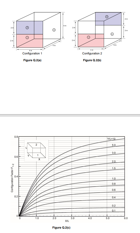
where surface $1$ ?is a radiator and surface $2$ ?is a window. In each case the

radiator is at a temperature of $340?,$ ?emissivity $0\mathrm{.}8$ ?and the window is a

temperature of $280?,$ ?emissivity $0\mathrm{.}7.$ ?All other surfaces in each

configuration could be treated as one black surface $(3)$ ?at temperature

$300?.$ ?It is required to calculate heat loss through the window for both

cases to determine the most energy efficient location for the radiator.

Assume the radiative heat transfer is the dominant heat transfer

mechanism.

Confiquration $1$

a$)$ ?Noting that, in configuration $1,$ ?surface $1$ ?and surface $2$ ?are on the

same wall, draw an electrical network that could be used to

calculate radiative heat transfer at each surface.

$[2$ ?marks$]$

b$)$ ?Calculate necessary configuration factors and resistances required

for the circuit drawn in $($a$).$

$[2$ ?marks$]$

c$)$ ?Use the network drawn in $($a$)$ ?to write nodal equations and solve

them to calculate heat transfer at surfaces $1,2$ ?and $3.$

$[3$ ?marks$]$

d$)$ ?Provide a heat balance to verify your answers obtained in $($c$).$

$[1$ ?mark$]$

Confiquration $2$

e$)$ ?Draw an electrical network to calculate radiative heat transfer at

surfaces of Configuration $2.$

$[2$ ?marks$]$

f$)$ ?Calculate necessary configuration factors required for the circuit

drawn in $($e$).$

$[2$ ?marks$]$

g$)$ ?Use the network drawn in $($e$)$ ?to write nodal equations and solve

them to calculate heat transfer at surfaces $1,2$ ?and $3.$

$[6$ ?marks$]$

h$)$ ?Provide a heat balance to verify your answers in $($g$).$

$[1$ ?mark$]$

i$)$ ?Based on your answers obtained in $($c$)$ ?and $($g$)$ ?what is the best

configuration to minimise heat transfer to the window. What is the

energy provided to the radiator in each case?

$[1$ ?mark$]$

Figure Q$\mathrm{.}2($c$)$ ?is to be used for configuration factor calculations.

Some useful configuration factor properties:Figure Q$\mathrm{.}2($c$)$

Configuration Factor F1.2 2 m 0.8 0.6 0.4 0.2 4m Configuration 1 Figure Q.2(a) 2 X 4m 2m 2m Configuration 2 Figure Q.2(b) 0 0 1.0 2.0 3.0 4.0 5.0 X/L Figure Q.2(c) Y/L-10 50 30 20 15 1.0 0.8 0.6 0.4 02 0.1 4m 6.0 2m 2m