

Barry Simkins Hardware store sells the Ace model electric drill . Daily demand for the drill is
Question:
Barry Simkin’s Hardware store sells the Ace model electric drill. Daily demand for the drill is relatively low but subject to some variability. Over the past 300 days, Simkin has observed the demand frequency shown in column 2 of Table 1 below. He converts this historical frequency into a probability distribution for the variable daily demand (column 3).
When Simkin places an order to replenish his inventory of drills, the time between when he places an order and when it is received (i.e. the lead time) is a probabilistic variable. Based on the past 100 orders, Simkin has found the lead time follows a discrete uniform distribution between one and three days. That is,
Lead time (days) | Probability |
1 2 3 | 1/3 1/3 1/3 |
He currently has seven (7) Ace electric drills in stock, and there are no orders due.
Simkin wants to identify the order quantity: Q and reorder point: R that will help him reduce his total monthly costs. The order quantity is the fixed size of each order that is placed. If the inventory level at the end of a day is at or below the reorder point R, an order is placed. The total cost includes the following components:
A fixed ordering cost that is incurred each time an order is placed.
A holding cost for each drill held in inventory from one period to the next.
A stockout cost for each drill that is not available to satisfy demand in a particular day.
Simkin estimates that the fixed cost of placing an order with his Ace drill supplier is $20. The cost of holding a drill in stock is $0.50 per drill per month. Assuming the shop operates 25 days each month on average, this translates to a holding cost of $0.02 per drill per day. Each time Simkin is unable to satisfy a demand (i.e., he has a stockout), the customer buys the drill elsewhere, and Simkin loses the sale. He estimates that the cost of a stockout is $8 per drill.
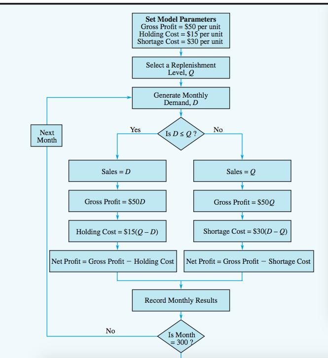
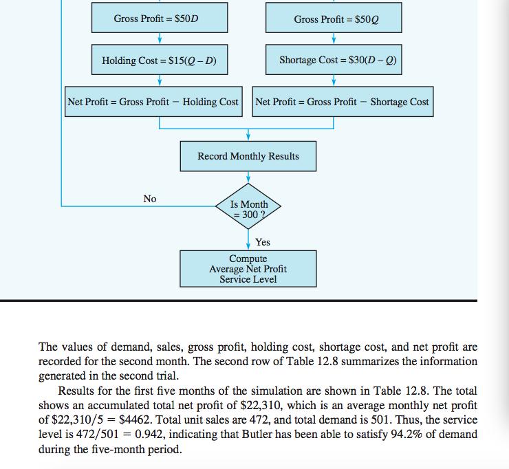
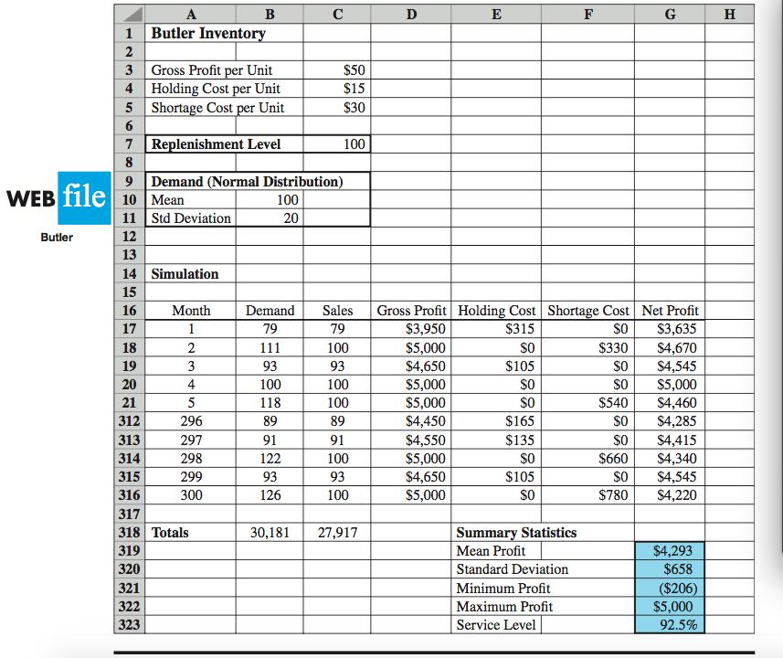
Note that there are two decision variables (order quantity, Q, and reorder point, R) and two probabilistic components (demand and lead time) in Simkin’s inventory problem. Using simulation, we can try different (Q, R) combinations (or policies) to see which combination yields the lowest total cost. Set up an Excel simulation model that will help SHS estimate the total cost for an inventory policy that has Q = 10 and R = 5; that is, each time the inventory position at the end of the day drops to five or fewer, we place an order for 10 drills with supplier. Simulate 100 days of operation. Your simulation should keep track of the following quantities: Beginning inventory, units received, available inventory, demand filled, ending inventory, stockouts, whether an order is placed or not, lead time and when the order arrives. Follow the BUTLER inventory problem (section 12.2 page 563) in your textbook.
Table 1: Distribution of Daily Demand for Ace Electric Drills
Demand for Drills | Frequency | Probability |
0 | 15 | 15/300 = 0.05 |
1 | 30 | 30/300 = 0.10 |
2 | 60 | 60/300 = 0.20 |
3 | 120 | 120/300 = 0.40 |
4 | 45 | 45/300 = 0.15 |
5 | 30 | 30/300 = 0.10 |
Total | 300 | 300/300 = 1.00 |
Your simulation should include the information summarized in the following tables (split into 2 tables for convenience). Note: Inventory position = Inventory on hand + Inventory on order (but not yet received). The 2 random inputs are demand and lead time.
A | B | C | D | E | F | G |
Day | Beginning inventory | Units received | Available inventory | Demand | Demand filled | Ending inventory |
1 2 etc. | 7 4 - | 0 0 - | 7 4 - | 3 3 - | 3 3 - | 4 1 - |
H | I | J | K | L | M | N | O |
Stockout | Inventory position | Place order? Yes =1; No = 0 | Lead time | Order arrive on day | Inventory cost | Stockout cost | Order cost |
0 0 etc. | 4 11 - | 1 0 - | 2 0 - | 4 0 - | $0.08 $0.02 - | $0 $0 - | $20 $0 - |
Total | |||||||
Total monthly cost | |||||||
Note: The numbers in the above tables are shown as examples and may not be the same in your spreadsheet simulation.
Please shown how to use excel solve question, For each spreadsheet, show only the first five and last five trials of your simulation. For example, if the number of simulation trials required is 1000, show only trials 1 to 5 and 996 to 1000 by hiding the intermediate trials from 6 to 995.
Expert Answer:


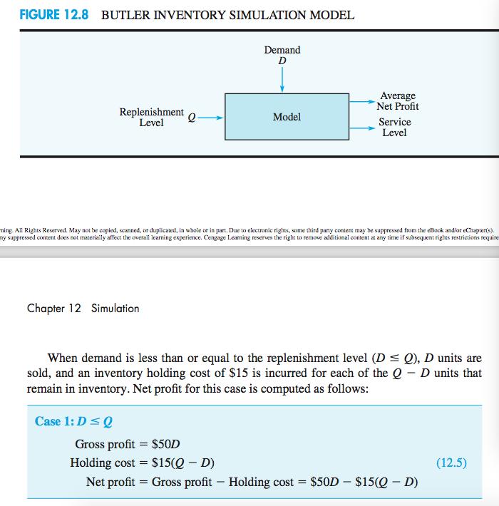
Operations Management Creating Value Along the Supply Chain
ISBN: 978-0470525906
7th Edition
Authors: Roberta S. Russell, Bernard W. Taylor
