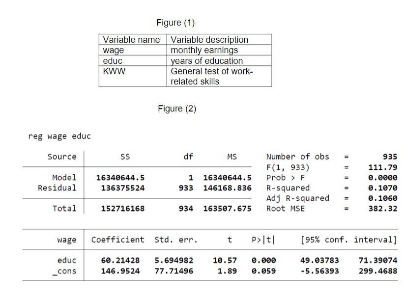
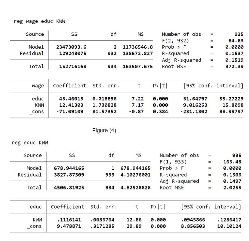
2. The variable descriptions and Stata outputs from the simple and multiple linear regression are available in the exam handout file. Use this file to answer the following questions. a. Firstly, report the results from the regression of wage on educ in the form of a fitted line, with the standard error of coefficients presented in parentheses underneath the corresponding coefficients. Round the numbers to two decimal places. [4 marks] b. Is the coefficient of educ statistically significant? [3 marks] c. Now consider the multiple linear regression that includes KWW as one of the explanatory variables. Between this regression and the simple linear regression in part (a), which model is more likely to measure the ceteris paribus effect of education on wages? Explain and when possible use evidence to support your answer. [8 marks] d. What happened to the standard error of educ after adding KWW to the model? Discuss. [10 marks] e. Do you agree or disagree with the following statement? "If the log of the dependent variable appears in the regression, changing the unit of measurement of any independent variable affects both the slope and intercept coefficients". Discuss [5 marks] reg wage educ Source Model Residual Total Figure (1) Variable name Variable description monthly earnings years of education General test of work- related skills wage educ KWW SS 16340644.5 136375524 152716168 Figure (2) 60.21428 146.9524 df 16340644.5 1 933 146168.836 934 wage Coefficient std. err. educ _cons MS 5.694982 77.71496 163507.675 Number of obs F(1, 933) Prob > F R-squared Adj R-squared Root MSE t P>|t| 10.57 0.000 1.89 0.059 11 49.03783 -5.56393 |||||| |||| 935 111.79 0.0000 0.1070 0.1060 382.32 [95% conf. interval] 71.39074 299.4688 reg wage educ KWW Source Model Residual Total Total SS wage Coefficient educ KWW _cons educ 23473093.6 129243075 KWW _cons 152716168 reg educ KWW Source Model 678.944165 Residual 3827.87509 SS df 4506.81925 43.46013 6.018896 12.41303 1.730828 -71.09109 81.57352 11736546.8 2 932 138672.827 934 Std. err. Figure (4) df MS Coefficient std. err. 163507.675 .1116141 .0086764 9.478871 .3171285 678.944165 1 933 4.10276001 t P>|t| MS 934 4.82528828 Number of obs F(2, 932) Prob > F R-squared 7.22 0.000 7.17 0.000 -0.87 0.384 Adj R-squared Root MSE t P>|t| 12.86 0.000 29.89 0.000 31.64797 9.016253 -231.1802 |||||||| 11 11 [95% conf. interval] 55.27229 15.8098 88.99797 Number of obs = F(1, 933) Prob > F R-squared Adj R-squared Root MSE .0945866 8.856503 |||||||||| = = 935 84.63 0.0000 0.1537 0.1519 372.39 = 935 165.48 0.0000 0.1506 0.1497 2.0255 [95% conf. interval] .1286417 10.10124