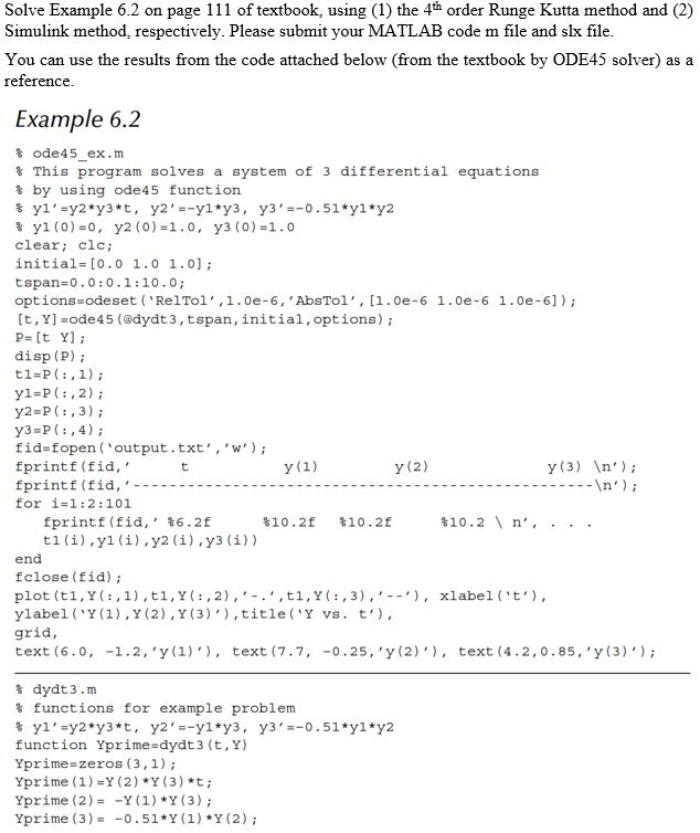
Solve Example 6.2 on page 111 of textbook, using (1) the 4th order Runge Kutta method and (2) Simulink method, respectively. Please submit your MATLAB code m file and slx file You can use the results from the code attached below (from the textbook by ODE45 solver) as a reference Example 6.2 ode45 ex.m % This program solves a system of 3 differential equations % by using ode45 function % y1 (0)=0, y2 (0)=1.0, y3 (0)=1.0 clear; clc initial [0.0 1.0 1.0] tspan 0.0:0.1:10.0; options-odeset ('RelTol',1.0e-6, 'AbsTol', [1.0e-6 1.0e-6 1.0e-6]) [t, Y] ode45 (@dydt3,tspan, initial,options) disp (P) y1 P(,2) y2-P(:,3) y3 P:,4) fid-fopen (output.txt,'w) fprintf (fid,' y (2) y (3) n') for i=1 :2 : 101 fprintf (fid,' %6.2f %10.2f %10.2f 10.2 \ n' end fclose (fid)i plot (tl, Y(),t1,Y(, 2),'-.',ti,Y:,3),), xlabelt, ylabel (Y(1),Y (2), Y (3)),titleY vs. t grid, text (6.o, -1.2, 'y (1), text (7.7, -0.25, 'y (2), text (4.2,0.85, 'y (3) % dydt3.m % functions for example problem function Yprime-dydt3 (t, Y) Yprime-zeros (3,1) Yprime (1)-Y (2) Y (3) t; yprime (2)--Y(1)*Y (3); Yprime (3)-0.51*Y (1) Y (2)