Solve the Below nonlinear model matlab code and to determine if the results shown in Figure 3.9 to 3.14 can be reproduced by adjusting the appropriate parameters.

Show the matlab plot generated and the corresponding code used to generate fig 3.9 and 3.14

% % Dynamic simulation of a nonsiothermal CFSTR. % Refer to Chapter 3 in Chemical Reactor Design & Control by W L Luyben % clear clc % % Initial concentration of specie A, kmol/cu.m. % ca0 = 8.01; % % Frequency factor for the first-order rate constant,1/s % k0 = 20.75E+06; % % Energy of activation, J/kmol % e = 69.71E+06; % % Initial reactor temperature, K % t0 = 294; % % Initial inlet temperature of the coolant, K % tcin = 294; % % Overall heat transfer coefficient, J/sq.m.-K-s % u = 851; taum = 60; % % Heat of Reaction, J/kmol % lamda = -69.71e+06; % % Density of process fluid, kg/cu.m. % roe = 801; % % Molecular weight of the process fluid % m = 100; % % Heat capacity of the process fluid, J/kg-K % cp = 3137; % % Heat capacity of the coolant, J/kg-K % cj = 4183; % % Density of the coolant, kg/cu.m. % roej = 1000; % % Define the fractional conversion. Change this value according to % the case that is being investigated % conversion = 0.85; % % Define the reactor temperature, K. Change this value as needed for % the case that is being investigated % tr = 350; % % Define the base-case feed rate, cu.m./s % f = 4.377E-03; % % Evaluate the exit concentration from the given ca0 & conversion % ca = ca0 * ( 1 - conversion ); % % Evaluate the first-order rate constant at the given reactor temperature % k = k0 * exp(-e/tr/8314); % % Evaluate the final value of the reactor volume % vr = f *(ca0 - ca)/k/ca; % % Evaluate the reactor diameter from the given volume % d = (2 * vr / pi)^(1/3); % % Evaluate the jacket cross-sectional area % areaj = 2 * pi * d^2; % % Evaluate the first term on the RHS of dCA/dt % q = (ca0 - ca)*f *(-lamda) - cp*roe*f*(tr-t0); tj = tr - q/u/areaj; vj = areaj/3; fj = q/(cj*(tj - tcin))/roej; vj = 0.1 * areaj; tjss = tj; fjss = fj; cass = ca; trss = tr; kss = k; fss = f; % % Controller gain and integral settings for 350K and 85% case; Alter these % as needed for the other cases. See Chapter 3 in Luyben for the precise % values % kc = 2.67; taui = 2709; fnew = fss * 1.2; % % Initial conditions and parameters % tstop = 4 * 3600; np = 0; erint = 0; tplot = 0; ca = cass; tj = tjss; tr = trss; time = 0; delta = 5; sp = trss; trlag1 = trss; trlag2 = trss; % % Integration loop % while time  1; op=1; end; if op == 1; end; if op  900; f = fnew; end; if time>=tplot; np = np + 1; % % Convert the integration time from secs to minutes for plotting purposes % timep(np)= time/60; trp(np) = tr; tjp(np) = tj; fjp(np) = fj; cap(np) = ca; tplot = tplot + 30; end q = u * areaj * (tr - tj); k = k0 * exp(-e/tr/8314); % % Derivative evaluations. Refer to the model ODE's to see the forms % dca = f*(ca0 - ca)/vr - k*ca; dtj = fj*(tcin - tj)/vj + q /(cj*roej*vj); dtr = f*(t0 - tr)/vr - lamda*k*ca/roe/cp - q/(cp*roe*vr); % % These next two ode's define the instrument and control valve lags as % simple firt-order system responses using the indicated time constant % Note that the first lag is the difference between the reactor temperature % and the lag associated with the controller outout while the second lag is % the difference between the controller output and the flow control valve % used to control the flow of the coolant % dtrlag1 = (tr - trlag1)/taum; dtrlag2 = (trlag1 - trlag2)/taum; % % Integration step % time = time + delta; ca = ca + dca*delta; tr = tr + dtr*delta; tj = tj + dtj*delta; trlag1 = trlag1 + dtrlag1*delta; trlag2 = trlag2 + dtrlag2*delta; % % Anti-reset windup (only integrate if the op parameter is between 0 & 1 % if op  0 erint = erint + error * kc * delta/taui; end; end; end; % % The next command 'clf' clears the plotting area % clf; % % Create the various subplots so they can be arranged in a 2 by 2 grid % % Plot the reactor temperature vs time % subplot(2,2,1); plot(timep,trp); grid; ylabel('TR, K'); % % Change the title for each case as needed % title('350 K at 85% Conversion with a 20% Increase in the Feed'); % % Plot the temperature of the reactor jacket coolant vs time % subplot(2,2,3); plot(timep,tjp); grid; ylabel('TJ, K)'); xlabel('Time, min'); % % Plot the flow rate of the reactor coolant % subplot(2,2,2); plot(timep,fjp); grid; ylabel('cu m/sec)') % % Plot the concnetration of specie A vs time % subplot(2,2,4); plot(timep,cap); grid; ylabel('CA, kmol/cu m)'); xlabel('Time, min');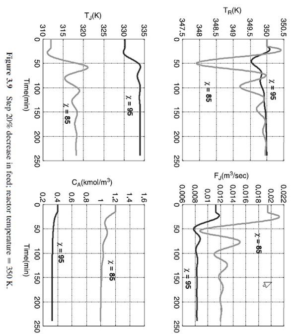 

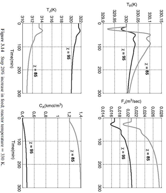
Figure 3.9 Step 20% decrease in feed; reactor temperature =350K. Figure 3.14 Step 20% increase in feed; reactor temperature =330K