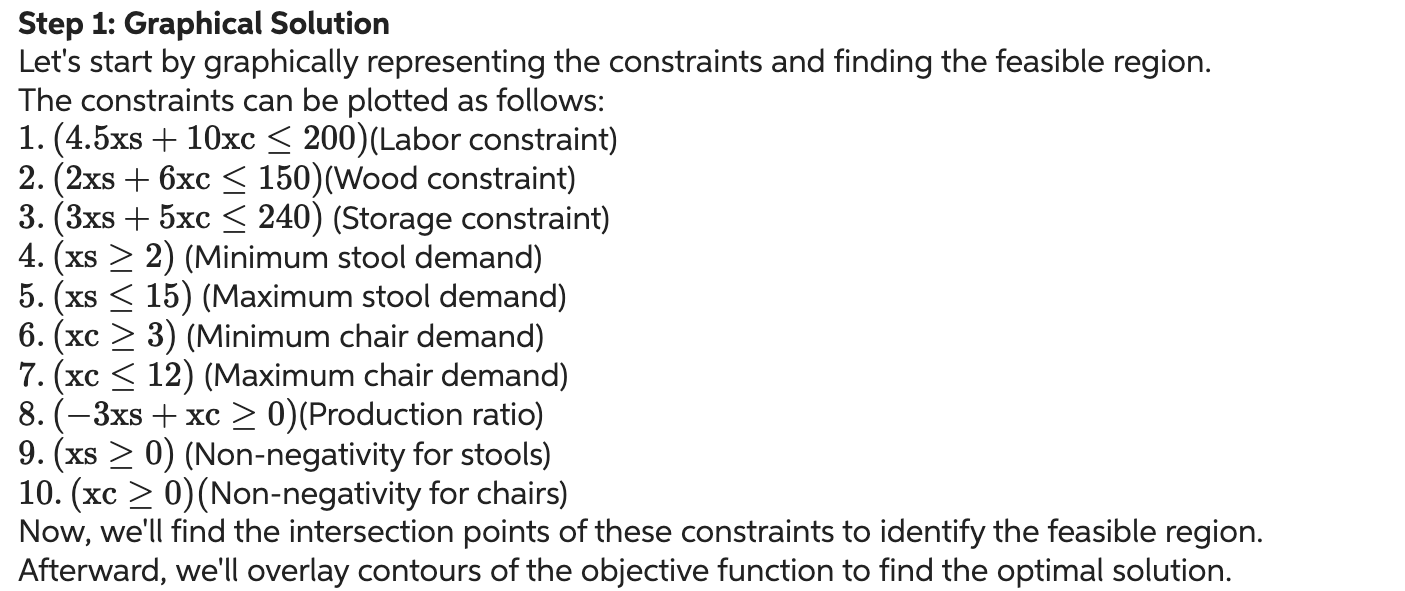
Question: Step 1: Graphical Solution Let's start by graphically representing the constraints and finding the feasible region. The constraints can be plotted as follows: 1.

Step 1: Graphical Solution Let's start by graphically representing the constraints and finding the feasible region. The constraints can be plotted as follows: 1. (4.5xs + 10xc 200) (Labor constraint) 2. (2xs + 6xc 150) (Wood constraint) 3. (3xs + 5xc 240) (Storage constraint) 4. (xs > 2) (Minimum stool demand) 5. (xs 15) (Maximum stool demand) 6. (xc 3) (Minimum chair demand) 7. (xc 12) (Maximum chair demand) 8. (3xs + xc 0)(Production ratio) 9. (xs 0) (Non-negativity for stools) 10. (xc > 0) (Non-negativity for chairs) Now, we'll find the intersection points of these constraints to identify the feasible region. Afterward, we'll overlay contours of the objective function to find the optimal solution.
Step by Step Solution
There are 3 Steps involved in it

Get step-by-step solutions from verified subject matter experts


