Step $1.$ In MATLAB, type "simulink" in the command window. Then go to "Blank Model" and save the model as $"$RLC$."$ We are going to create the model show in Fig. $2$ to model an RLC circuit with a square wave input.

Step $2.$ Click on the Library Browser $$ Simulink $$ Sources and drag a Pulse Generator into the blank model page. Set the amplitude to $1$ and period to $\frac{1}{523}$ seconds $(523$ Hz $)$ with $50\%$ duty cycle to create a standard square wave. This frequency is chosen so that the $3^{rd}$ harmonic is approximately in the center of the RLC bandpass $($however$,$ other harmonics will get through this filter as it is not very narrow$).$

Step $3.$ Go back to the Library Browser $$ Simulink $$ Continuous block set and drag a Transfer Fcn block onto the workspace figure. Click on the transfer function block and enter the RLC circuit parameters from Eq$.(4).$ Drag the arrow head form the Pulse Generator to the Transfer Fon Block. If you increase the size of the Transfer Fcn block, you will see the equation as shown in Fig. $2.$

Step $4.$ Go to bibrary Browser $$ Simulink $$ Sinks in the Simulink Library Browser and drag a scope and a To Workspace $($simout$)$ block to the figure. Connect those in parallel to the output of the Transfer Fcn block. To connect the second block $($simout$)$ to the output of the Transfer Fcn$,$ click on the input arrow of the second block and drag it backwards to the line leading to the first block $($Scope$).$ Click on the simout block and rename the output variable if desired and select Save format to be Structure with Time.

Step $5.$ Go to the top level tab "MODELING" and then the gear icon $($Model Settings$)$ and under Solver $$ Solver details change the Relative Tolerance to $1e-6.$ Set the Stop time to be $\mathrm{.}01$ seconds. Start the simulation by pressing the "Run" button on the tool bar. You can view the output by clicking on the scope icon. You may need to adjust the axes scaling to get a good display. On the scope you can go to Tools $$ Axis Scaling $$ Automatically Scale Axis Limits. Provide a screen capture of your scope output.

Step $6.$ You can go to the workspace and look for your output variable $($out$.$simout$).$ You can plot the output using this command: plot$($out$.$simout.time, out.simout.signals.values$).$ Provide a copy of the resulting figure $($be sure to label axes and add units to your plot$).$Step $8.$ Plot the input and output versus time using a command like this:

plot$($ out.motorin.Time, out.motorin.data, $\text{'}$b$-\text{'},$ out.motorout.Time, out.motorout.data, $\text{'}$r$-\text{'})$

Add a grid, legend, axis labels with units, and a title. Note that the output units are radians $($angle of motor axle$).$ We are modeling a big heavy motor that appears to be taking about $10$ seconds to rotate once with the pulse train input we are applying. It should be clear from the plot that the motor rotation in radians is not following the input voltage. Thus, we need a negative feedback close loop control system.

$4\mathrm{.}3$ Simulating the negative feedback closed$-$loop DC motor

Figure $4$: DC motor with negative feedback closed$-$loop control and a proportional controller $($i$.$e$.,$ the gain of $5$ amplifier block$).$Step $8.$ Create a new model named ClosedLoop as shown in Fig. $4.$ This an example of a negative feedback closed$-$loop control system with a proportional controller $($i$.$e$.,$ the gain of $5$ amplifier block in Fig. $4).$ Set the period of the square wave to be $10$ seconds with $50\%$ duty cycle and use a simulation Stop time of $50$ seconds. You will need the Math block set to get the summation block. Note the gain block added as well $($shown with a gain of $5).$ Rename the input and output variables as shown in Fig. $4.$

Step $9.$ Run the simulation and view the input and output. Note that the motor output should approximate the control signal input $($unlike before when the motor just rotated in one direction continuously$).$ Try gains values of $0\mathrm{.}1,0\mathrm{.}5,1,2,10,$ and $20.$ Comment on what you observe as the impact of the gain on the motor output and how well it follows the control signal.

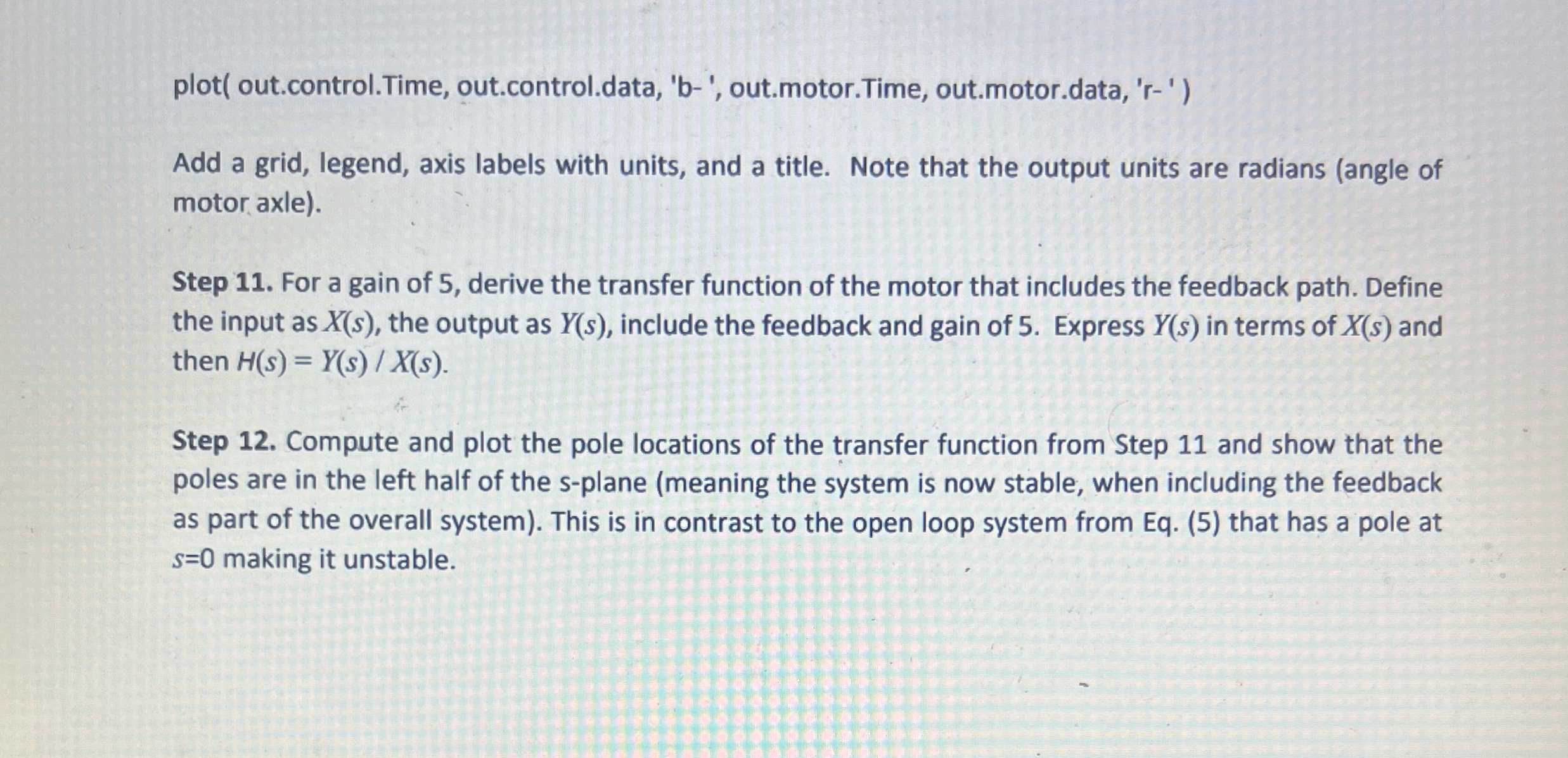
Step $10.$ Pick the gain that you think works the best and provide plot of the control and motor output using a command like thisplot$($ out.control.Time, out.control.data, $\text{'}$b$-\text{'},$ out.motor.Time, out.motor.data, $\text{'}$r$-\text{'})$

Add a grid, legend, axis labels with units, and a title. Note that the output units are radians $($angle of motor axle$).$

Step $11.$ For a gain of $5,$ derive the transfer function of the motor that includes the feedback path. Define the input as $x(s),$ the output as $Y(s),$ include the feedback and