step by step plis

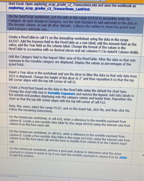
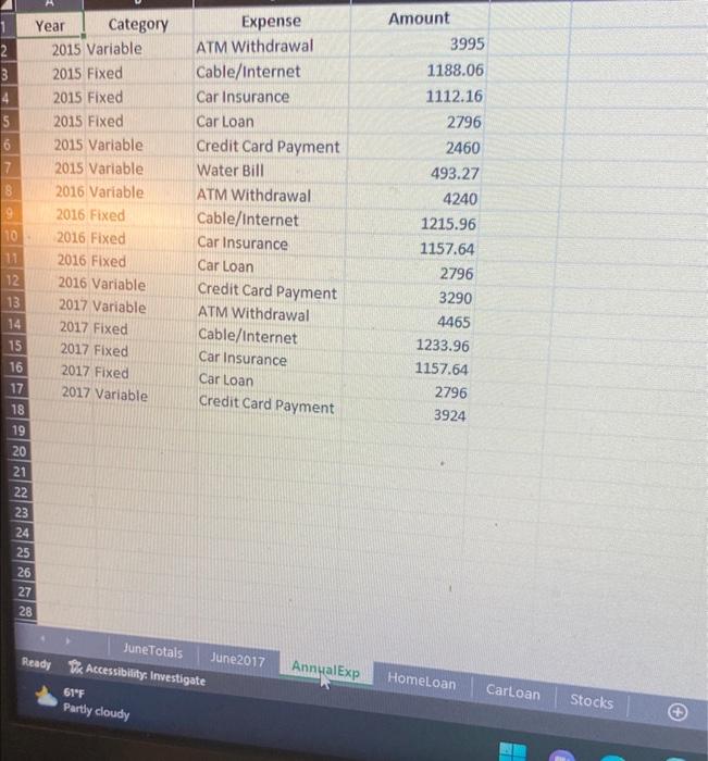
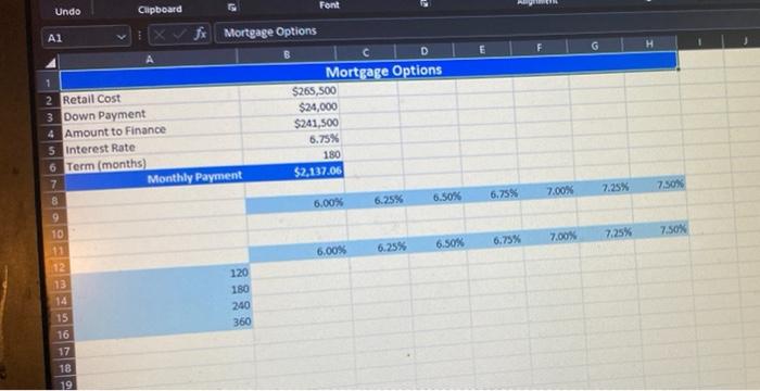
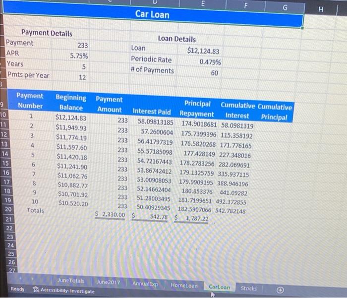
Start Excel. Open exploring_ecap_grader_____ Transactions.xlsx and save the workbook as exploring_ecap_grader_c2_Transactions_LastFirst. On the JuneTotals worksheet, sort the data in the range A3:E16 in ascending order by Category. At each change in Category, use the Sum function to add subtotals to the data in the Amount column. Accept all other defaults. Collapse the outline to show the grand total and Category subtotals only. Create a PivotTable in cell F1 on the Annual Exp worksheet using the data in the range A1:D17. Add the Expense field to the PivotTable as a row label; add the Amount field as the value; add the Year field as the column label. Change the format of the values in the PivotTable to accountina with no decimal places and set columns F:J to AutoFit Column Width. Add the Category field to the Report Filter area of the PivotTable. Filter the data so that only expenses in the Variable category are displayed. Display the values as percentages of the grand total. Insert a Year slicer in the worksheet and use the slicer to filter the data so that only data from 2015 is displayed. Change the height of the slicer to 2 and then reposition it so that the top left corner aligns with the top left corner of cell 12 . Create a PivotChart based on the data in the PivotTable using the default Pie chart type. Change the chart title text to Variable Expenses and remove the legend. Add data labels to the outside end position displaying only the category names and leader lines. Reposition the chart so that the top left corner aligns with the top left corner of cell F13. Note, Mac users, select the range FS:G7, and on the Insert tab, click Pie, and then dick Pie. Follow the remaining instructions. On the HomeLoan worksheet, in cell A10, enter a reference to the monthly payment from column B. Create a one-variable data table for the range A9:H10 using the interest rate from column B as the Row input cell. On the Homeloan worksheet, in cell A12, enter a reference to the monthly payment from column B. Create a two-variable data table in the range A12:H16, using the interest rate from column B as the Row input cell and the term in months from column B as the Column input cell. On the Homeloan worksheet, perform a goal seek analysis to determine what the down payment in column B needs to be if you want the monthly payment in column B to be 2000 . Accept the solution. Step Instructions \begin{tabular}{|ll|l|} \hline Postion: & Serch results \\ \hline \end{tabular} Stock Purchases \begin{tabular}{c|c|c|c|c|c|} A & B & C & D & E & F \\ \hline Stock Purchases \end{tabular} COMPANY Start Excel. Open exploring_ecap_grader_____ Transactions.xlsx and save the workbook as exploring_ecap_grader_c2_Transactions_LastFirst. On the JuneTotals worksheet, sort the data in the range A3:E16 in ascending order by Category. At each change in Category, use the Sum function to add subtotals to the data in the Amount column. Accept all other defaults. Collapse the outline to show the grand total and Category subtotals only. Create a PivotTable in cell F1 on the Annual Exp worksheet using the data in the range A1:D17. Add the Expense field to the PivotTable as a row label; add the Amount field as the value; add the Year field as the column label. Change the format of the values in the PivotTable to accountina with no decimal places and set columns F:J to AutoFit Column Width. Add the Category field to the Report Filter area of the PivotTable. Filter the data so that only expenses in the Variable category are displayed. Display the values as percentages of the grand total. Insert a Year slicer in the worksheet and use the slicer to filter the data so that only data from 2015 is displayed. Change the height of the slicer to 2 and then reposition it so that the top left corner aligns with the top left corner of cell 12 . Create a PivotChart based on the data in the PivotTable using the default Pie chart type. Change the chart title text to Variable Expenses and remove the legend. Add data labels to the outside end position displaying only the category names and leader lines. Reposition the chart so that the top left corner aligns with the top left corner of cell F13. Note, Mac users, select the range FS:G7, and on the Insert tab, click Pie, and then dick Pie. Follow the remaining instructions. On the HomeLoan worksheet, in cell A10, enter a reference to the monthly payment from column B. Create a one-variable data table for the range A9:H10 using the interest rate from column B as the Row input cell. On the Homeloan worksheet, in cell A12, enter a reference to the monthly payment from column B. Create a two-variable data table in the range A12:H16, using the interest rate from column B as the Row input cell and the term in months from column B as the Column input cell. On the Homeloan worksheet, perform a goal seek analysis to determine what the down payment in column B needs to be if you want the monthly payment in column B to be 2000 . Accept the solution. Step Instructions \begin{tabular}{|ll|l|} \hline Postion: & Serch results \\ \hline \end{tabular} Stock Purchases \begin{tabular}{c|c|c|c|c|c|} A & B & C & D & E & F \\ \hline Stock Purchases \end{tabular} COMPANY