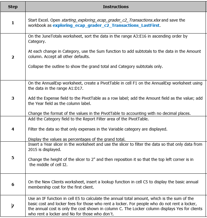
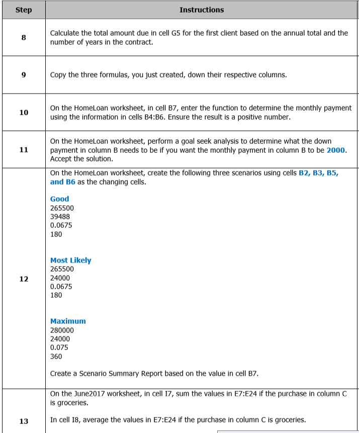
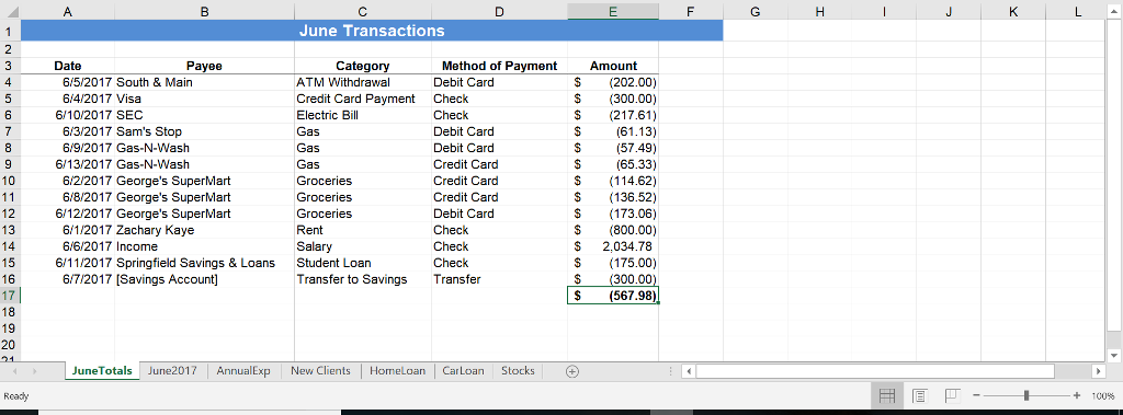
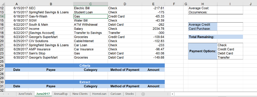
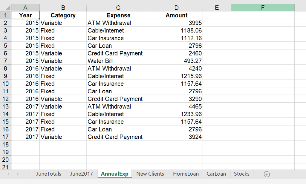
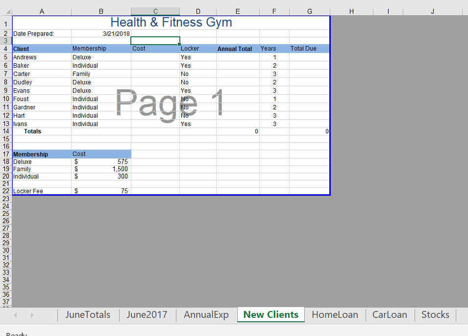
Step Instructions Start Excel. Open starting_exploring ecap_grader_c2_Transactions.xlsx and save the workbook as exploring_ecap_grader_c2_Transactions_LastFirst. On the JuneTotals worksheet, sort the data in the range A3:E16 in ascending order by Category At each change in Category, use the Sum function to add subtotals to the data in the Amount column. Accept all other defaults 2 Collapse the outline to show the grand total and Category subtotals only On the AnnualExp worksheet, create a PivotTable in cell F1 on the AnnualExp worksheet using the data in the range A1:D17. Add the Expense field to the PivotTable as a row label; add the Amount field as the value; add the Year field as the column label 3 Change the format of the values in the PivotTable to accounting with no decimal places Add the Category field to the Report Filter area of the PivotTable 4 Filter the data so that only expenses in the Variable category are displayed Display the values as percentages of the grand total Insert a Year slicer in the worksheet and use the slicer to filter the data so that only data from 2015 is displayed 5 Change the height of the slicer to 2" and then reposition it so that the top left corner is in the middle of cell 12 On the New Clients worksheet, insert a lookup function in cell C5 to display the basic annual membership cost for the first client. Use an IF function in cell E5 to calculate the annual total amount, which is the sum of the basic cost and locker fees for those who rent a locker. For people who do not rent a locker, the annual cost is only the cost shown in column C. The Locker column displays Yes for clients who rent a locker and No for those who don't