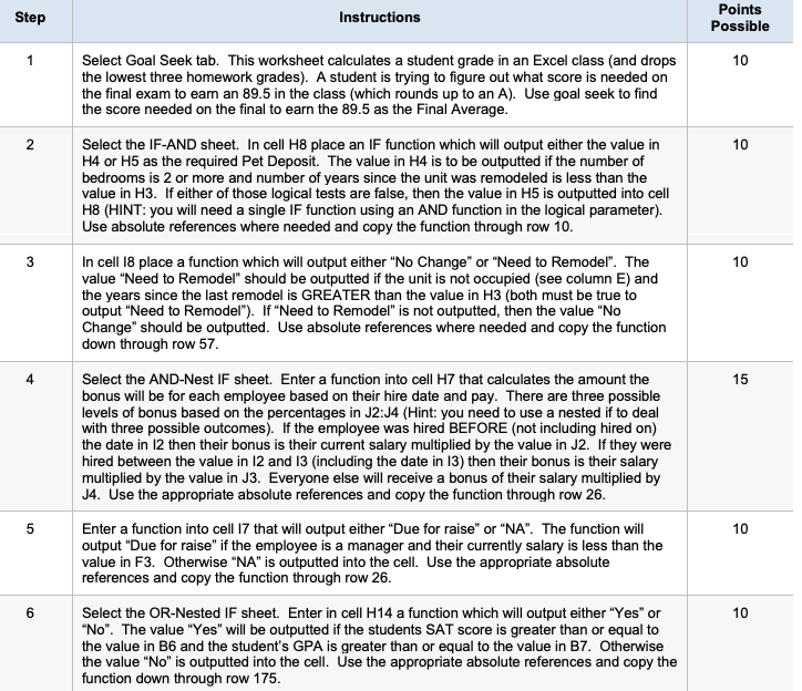
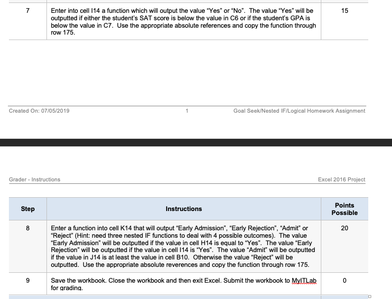
Question: Step Instructions Points Possible 1 10 N Select Goal Seek tab. This worksheet calculates a student grade in an Excel class (and drops the lowest

Step Instructions Points Possible 1 10 N SelectStep Instructions Points Possible 1 10 N Select

Step Instructions Points Possible 1 10 N Select Goal Seek tab. This worksheet calculates a student grade in an Excel class (and drops the lowest three homework grades). A student is trying to figure out what score is needed on the final exam to earn an 89.5 in the class (which rounds up to an A). Use goal seek to find the score needed on the final to earn the 89.5 as the Final Average. Select the IF-AND sheet. In cell H8 place an IF function which will output either the value in H4 or H5 as the required Pet Deposit. The value in H4 is to be outputted if the number of bedrooms is 2 or more and number of years since the unit was remodeled is less than the value in H3. If either of those logical tests are false, then the value in H5 is outputted into cell H8 (HINT: you will need a single IF function using an AND function in the logical parameter). Use absolute references where needed and copy the function through row 10. 10 3 10 4 15 In cell 18 place a function which will output either "No Change" or "Need to Remodel". The value "Need to Remodel" should be outputted if the unit is not occupied (see column E) and the years since the last remodel is GREATER than the value in H3 (both must be true to output "Need to Remodel"). If "Need to Remodel" is not outputted, then the value "No Change" should be outputted. Use absolute references where needed and copy the function down through row 57. Select the AND-Nest IF sheet. Enter a function into cell H7 that calculates the amount the bonus will be for each employee based on their hire date and pay. There are three possible levels of bonus based on the percentages in J2:34 (Hint: you need to use a nested if to deal with three possible outcomes). If the employee was hired BEFORE (not including hired on) the date in 12 then their bonus is their current salary multiplied by the value in J2. If they were hired between the value in 12 and 13 (including the date in 13) then their bonus is their salary multiplied by the value in J3. Everyone else will receive a bonus of their salary multiplied by J4. Use the appropriate absolute references and copy the function through row 26. Enter a function into cell 17 that will output either "Due for raise" or "NA". The function will output Due for raise" if the employee is a manager and their currently salary is less than the value in F3. Otherwise "NA" is outputted into the cell. Use the appropriate absolute references and copy the function through row 26. Select the OR-Nested IF sheet. Enter in cell H14 a function which will output either "Yes" or "No". The value "Yes" will be outputted if the students SAT score is greater than or equal to the value in B6 and the student's GPA is greater than or equal to the value in B7. Otherwise the value "No" is outputted into the cell. Use the appropriate absolute references and copy the function down through row 175. 5 10 6 10 7 15 Enter into cell 114 a function which will output the value "Yes" or "No". The value "Yes" will be outputted if either the student's SAT score is below the value in C6 or if the student's GPA is below the value in C7. Use the appropriate absolute references and copy the function through row 175. Created On: 07/05/2019 1 Goal Seek/Nested IF/Logical Homework Assignment Grader - Instructions Excel 2016 Project Step Instructions Points Possible 8 20 Enter a function into cell K14 that will output "Early Admission", "Early Rejection", "Admit" or "Reject" (Hint: need three nested IF functions to deal with 4 possible outcomes). The value "Early Admission" will be outputted if the value in cell H14 is equal to "Yes". The value "Early Rejection" will be outputted if the value in cell 114 is "Yes". The value "Admit" will be outputted if the value in J14 is at least the value in cell B10. Otherwise the value "Reject" will be outputted. Use the appropriate absolute reverences and copy the function through row 175. 9 0 Save the workbook. Close the workbook and then exit Excel. Submit the workbook to MyITLab for grading. Step Instructions Points Possible 1 10 N Select Goal Seek tab. This worksheet calculates a student grade in an Excel class (and drops the lowest three homework grades). A student is trying to figure out what score is needed on the final exam to earn an 89.5 in the class (which rounds up to an A). Use goal seek to find the score needed on the final to earn the 89.5 as the Final Average. Select the IF-AND sheet. In cell H8 place an IF function which will output either the value in H4 or H5 as the required Pet Deposit. The value in H4 is to be outputted if the number of bedrooms is 2 or more and number of years since the unit was remodeled is less than the value in H3. If either of those logical tests are false, then the value in H5 is outputted into cell H8 (HINT: you will need a single IF function using an AND function in the logical parameter). Use absolute references where needed and copy the function through row 10. 10 3 10 4 15 In cell 18 place a function which will output either "No Change" or "Need to Remodel". The value "Need to Remodel" should be outputted if the unit is not occupied (see column E) and the years since the last remodel is GREATER than the value in H3 (both must be true to output "Need to Remodel"). If "Need to Remodel" is not outputted, then the value "No Change" should be outputted. Use absolute references where needed and copy the function down through row 57. Select the AND-Nest IF sheet. Enter a function into cell H7 that calculates the amount the bonus will be for each employee based on their hire date and pay. There are three possible levels of bonus based on the percentages in J2:34 (Hint: you need to use a nested if to deal with three possible outcomes). If the employee was hired BEFORE (not including hired on) the date in 12 then their bonus is their current salary multiplied by the value in J2. If they were hired between the value in 12 and 13 (including the date in 13) then their bonus is their salary multiplied by the value in J3. Everyone else will receive a bonus of their salary multiplied by J4. Use the appropriate absolute references and copy the function through row 26. Enter a function into cell 17 that will output either "Due for raise" or "NA". The function will output Due for raise" if the employee is a manager and their currently salary is less than the value in F3. Otherwise "NA" is outputted into the cell. Use the appropriate absolute references and copy the function through row 26. Select the OR-Nested IF sheet. Enter in cell H14 a function which will output either "Yes" or "No". The value "Yes" will be outputted if the students SAT score is greater than or equal to the value in B6 and the student's GPA is greater than or equal to the value in B7. Otherwise the value "No" is outputted into the cell. Use the appropriate absolute references and copy the function down through row 175. 5 10 6 10 7 15 Enter into cell 114 a function which will output the value "Yes" or "No". The value "Yes" will be outputted if either the student's SAT score is below the value in C6 or if the student's GPA is below the value in C7. Use the appropriate absolute references and copy the function through row 175. Created On: 07/05/2019 1 Goal Seek/Nested IF/Logical Homework Assignment Grader - Instructions Excel 2016 Project Step Instructions Points Possible 8 20 Enter a function into cell K14 that will output "Early Admission", "Early Rejection", "Admit" or "Reject" (Hint: need three nested IF functions to deal with 4 possible outcomes). The value "Early Admission" will be outputted if the value in cell H14 is equal to "Yes". The value "Early Rejection" will be outputted if the value in cell 114 is "Yes". The value "Admit" will be outputted if the value in J14 is at least the value in cell B10. Otherwise the value "Reject" will be outputted. Use the appropriate absolute reverences and copy the function through row 175. 9 0 Save the workbook. Close the workbook and then exit Excel. Submit the workbook to MyITLab for grading

Step by Step Solution

There are 3 Steps involved in it

1 Expert Approved Answer
Step: 1 Unlock blur-text-image
Question Has Been Solved by an Expert!

Get step-by-step solutions from verified subject matter experts

Step: 2 Unlock
Step: 3 Unlock

Students Have Also Explored These Related General Management Questions!