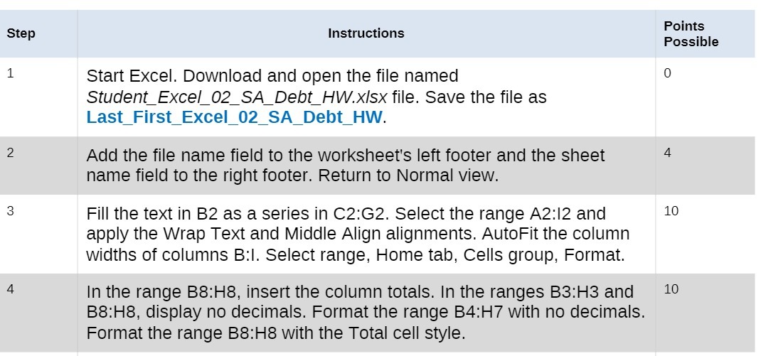
Question: Step Instructions Points Possible 1 Start Excel. Download and open the file named 0 Student_Excel_02_SA_Debt_HW.xIsx file. Save the file as Last First_Excel_02_SA_Debt_HW. 2 Add the

Step Instructions Points Possible 1 Start Excel. Download and open the file named 0 Student_Excel_02_SA_Debt_HW.xIsx file. Save the file as Last First_Excel_02_SA_Debt_HW. 2 Add the file name field to the worksheet's left footer and the sheet 4 name field to the right footer. Return to Normal view. Fill the text in B2 as a series in C2:G2. Select the range A2:12 and 10 apply the Wrap Text and Middle Align alignments. AutoFit the column widths of columns B:I. Select range, Home tab, Cells group, Format. 4 In the range B8:H8, insert the column totals. In the ranges B3:H3 and 10 B8:H8, display no decimals. Format the range B4:H7 with no decimals. Format the range B8:H8 with the Total cell style

Step by Step Solution

There are 3 Steps involved in it

1 Expert Approved Answer

Step: 1 Unlock blur-text-image

Question Has Been Solved by an Expert!

Get step-by-step solutions from verified subject matter experts

Step: 2 Unlock

Step: 3 Unlock

Students Have Also Explored These Related Accounting Questions!

Project Description: You have recently been elected social coordinator for your University's student government association. As part of your duties, you are required to plan an annual scholarship...

You and a business partner opened a fitness gym three years ago. Your partner oversees managing the operations of the gym, ensuring the right equipment is on hand, maintenance is conducted, and the...

Please help me do this excel assignment by providing me with very very specific instructions. Give me step by step of what to implement where using which tools. Step Instructions Points Possible 1...

Steps to Perform: Step Instructions Points Possible 1 Start Excel. Download and open the file named 0 Exp19_Excel_Ch01_ CapAssessment_ Training.xisx. Grader has automatically added your last name to...

Exp19_Excel_Ch05_HOEAssessment_Fine_Art Project Description: You are an analyst for a fine art dealer. Customers are especially fond of James C. Christensens art. You prepared a list of his artwork:...

Project Description: You manage several apartment complexes in Phoenix, Arizona. You created a dataset that lists details for each apartment complex, such as apartment number, including number of...

Using job order costing, determine the product unit cost based on the following costs incurred during March: liability insurance, manufacturing, $2,500; rent, sales office, $2,900; depreciation,...

A certain one-particle, one-dimensional system has = ae-ibte-bmx2/h, where a and b are constants and m is the particle's mass. Find the potential-energy function V for this system.

Contrast a rolling forecast with the master budget. Discuss the potential advantages of a rolling forecast. Question content area bottom Part 1 A . A rolling forecast involves will look at weekly...

Determine the major differences between U.S. GAAP and IFRS disclosure reporting requirements related to each separately reportable operating segment. Next, give your opinion as to whether either U.S....