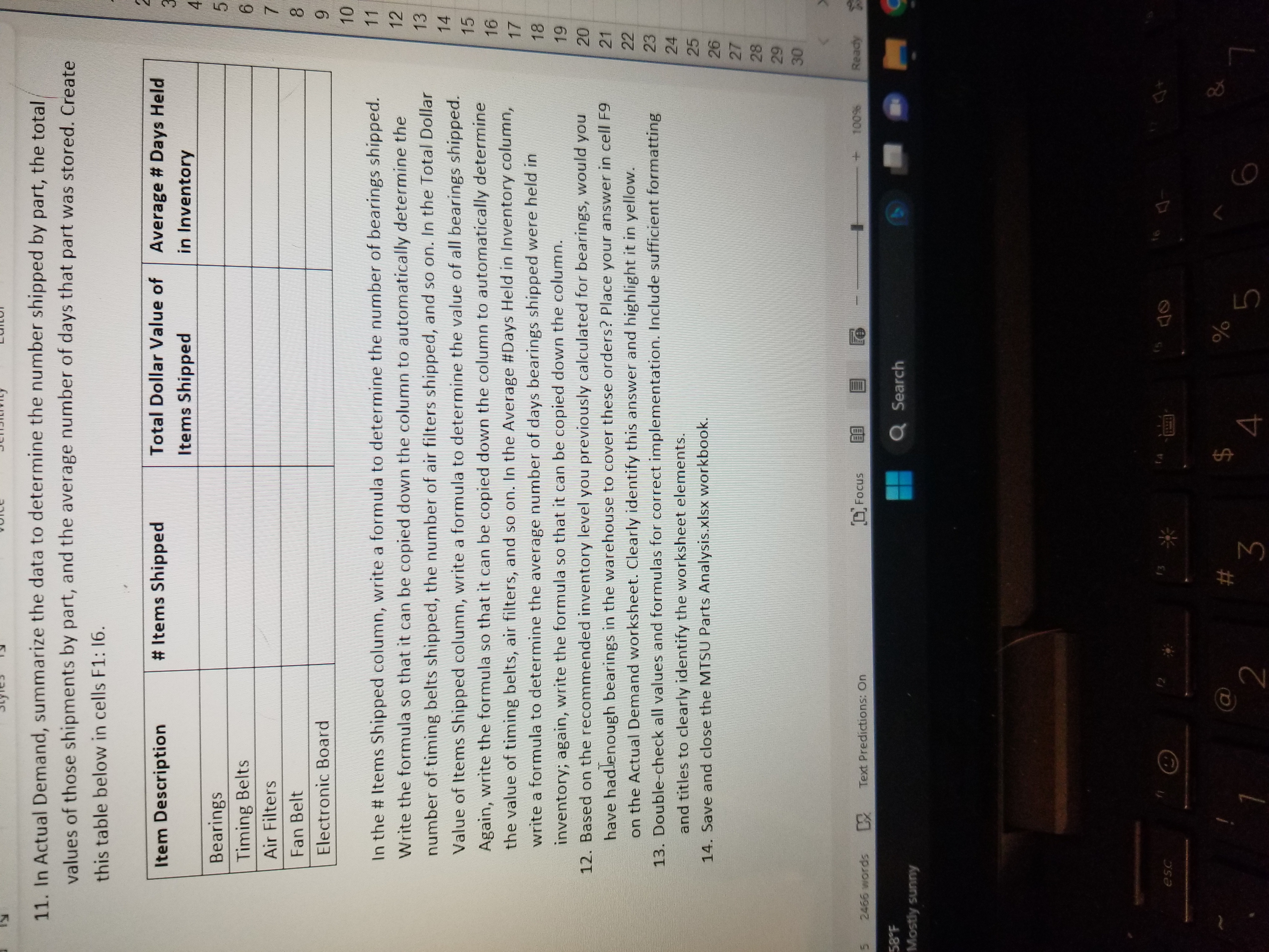
Styles IN Voice Sensitivity Editor 2. Modify the format of the data on the BearingData worksheet so that zero values are displayed with a 0 instead of the default dash, aligned on the right side of the column. 3. On the BearingData worksheet, take the existing 30-day data for these bearings for each customer to calculate the high and low limits of the bearing demand by customer. 4. On a new worksheet named "Simulation" (no quotes), use the high and low limits you just calculated to simulate daily requirements for each customer to obtain a combined daily requirement. In cell A3, enter "Day". Copy the customer numbers from the Bearing Data sheet and paste them in Simulation in cells B3-K3. In column A, starting in cell A4, create a numeric list of days (A4 will be 1, A5 will be 2, etc.) up to 240. Assume that the daily requirements will vary for each customer randomly between the high and low limits you have calculated from the existing 30-day data for that customer. Generate the data for 240 instances (days) for each customer in cells B4:K243. 5. Create a new worksheet named "Simulation Data 1" (no quotes). Set this up to look exactly like the Simulation worksheet - same customer numbers and days in the same cells. Copy the data you generated in Simulation cells B4:K243 as values (paste special - as values) to the same cells in Simulation Data 1. a. FYI - we copy and paste special the data because the function used to create these numbers will run (and update) every time you make a change to your workbook, changing the numbers. By pasting the values in another sheet, we prevent the accidental changing of the values generated. 19 6. On the Simulation Data 1 worksheet, in column L, calculate the total demand by day for the 10 20 customers in cells L4:1243. Use this daily demand total data to calculate the overall mean, 21 mode, median, and standard deviation for the combined requirements of all 10 customers in 22 23 cells P21:P24 respectively. Label the cells in 021:024. Use cell shading to clearly identify your 24 calculation area. 25 7. Generate a ranking of the data (1 to 240) in cells M4:M243 so that the day with the least total 26 demand has a rank of 1 (HINT: Use the RANK. EQ function). Put "rank" in cell M3. Again, use cell 27 shading to clearly identify columns with your calculations. 28 8 . Create a listing of the top (cells P4:P8) and bottom (cells Q4:08) five daily combined demands 29 from the simulated instances (HINT: Use the LARGE and SMALL formulas). Clearly identify this 30 listing wing hardors and chading 2466 words Text Predictions: On Focus 100% Ready Mostly sunny Q Search PSC 16ard Styles Ty Voice Sensitivity Editor 8. Create a listing of the top (cells P4:P8) and bottom (cells Q4:08) five daily combined demands from the simulated instances (HINT: Use the LARGE and SMALL formulas). Clearly identify this H6 listing using borders and shading. 9. Recommend a target inventory level needed for a five-day period based on the following: to be on the cautious side, assume each day's supply will be equal to the average daily demand for all locations combined, plus three standard deviations. Since the mean and standard CA WN deviations might not already be integers, round the daily demand up to the nearest whole number in your formula. Then, use this calculated daily demand (average plus 3 standard deviations) to calculate demand over a five-day period. Place this recommendation in cell P14, again clearly identifying it. Add the label Bearing Recommended to identify the cell containing the actual value. 9 10. The warehouse manager has tracked a total of five different parts over the past five days, 10 recording for each shipment the value of the part and the number of days it was in storage. One 11 of these tracked parts is the bearing you have just analyzed. The data has been compiled in a 12 workbook named Demand.xIsx. Each line item represents a single shipment of one item. Create 13 14 15 16 17 18 19 20 21 22 23 24 25 26 27 a new worksheet named "Actual Demand" (no quotes). Copy the data from the Demand.xIsx 28 workbook to Actual Demand. 29 11. In Actual Demand, summarize the data to determine the number shipped by part, the total 30 values of those chinmente hy nart and the average number of days that nart was stored Create of 5 2466 words CX Text Predictions: On Focus 10056 Ready Acce 58 F Q Search Mostly sunny 13 es.c 2 A 511. In Actual Demand, summarize the data to determine the number shipped by part, the total values of those shipments by part, and the average number of days that part was stored. Create this table below in cells F1: 16. Item Description # Items Shipped Total Dollar Value of Average # Days Held Items Shipped in Inventory Bearings Timing Belts Air Filters Fan Belt CO Electronic Board 9 10 In the # Items Shipped column, write a formula to determine the number of bearings shipped. 11 Write the formula so that it can be copied down the column to automatically determine the 12 number of timing belts shipped, the number of air filters shipped, and so on. In the Total Dollar 13 Value of Items Shipped column, write a formula to determine the value of all bearings shipped. 14 15 Again, write the formula so that it can be copied down the column to automatically determine 16 the value of timing belts, air filters, and so on. In the Average #Days Held in Inventory column, 17 write a formula to determine the average number of days bearings shipped were held in 18 inventory; again, write the formula so that it can be copied down the column. 19 12. Based on the recommended inventory level you previously calculated for bearings, would you 20 have hadlenough bearings in the warehouse to cover these orders? Place your answer in cell F9 21 on the Actual Demand worksheet. Clearly identify this answer and highlight it in yellow. 22 13. Double-check all values and formulas for correct implementation. Include sufficient formatting 23 and titles to clearly identify the worksheet elements. 24 14. Save and close the MTSU Parts Analysis.xisx workbook. 25 26 27 28 29 30 2466 words CX Text Predictions: On FOCUS 1009% Ready 58 F Q Search Mostly sunny esc 12 13 5