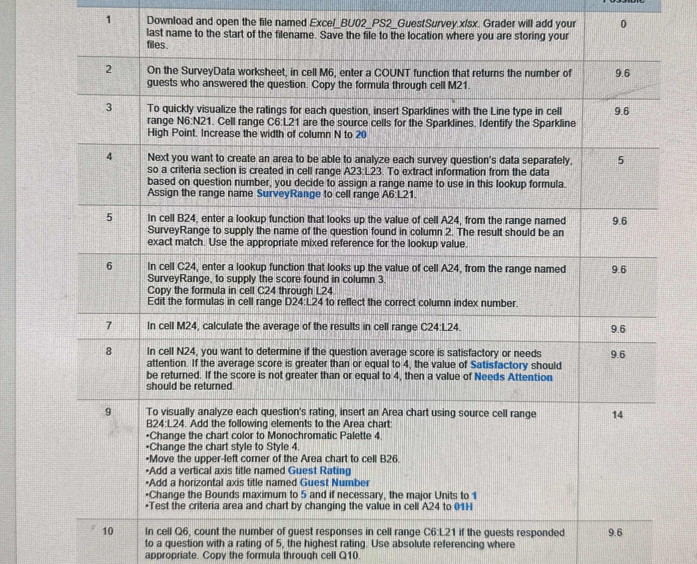
$\backslash$table$[[1,\backslash$table$[[$Download and open the file named Excel$\_$BU$02\_$PS$2\_$GuestSurvey.xlsx$.$ Grader will add your$],[$last name to the start of the filename. Save the file to the location where you are storing your$],[$files$.]],0],[2,\backslash$table$[[$On the SurveyData worksheet, in cell M$6,$ enter a cOUNT function that returns the number of$],[$guests who answered the question. Copy the formula through cell M$21.]],9\mathrm{.}6],[3,\backslash$table$[[$To quickly visualize the ratings for each question, insert Sparklines with the Line type in cell$],[$range N$6$:N$21.$ Cell range C$6$:L$21$ are the source cells for the Sparkines. Identify the Sparkine$],[$High Point. Increase the width of column N to $20]],9\mathrm{.}6],[4,\backslash$table$[[$Next you want to create an area to be able to analyze each survey question's data separately,$],[$so a criteria section is created in cell range A$23\mathrm{.}123.$ To extract information from the data$],[$based on question number, you decide to assign a range name to use in this lookup formula.$],[$Assign the range name SurveyRange to cell range A$6$:L$21.]],5],[5,\backslash$table$[[$In cell B$24,$ enter a lookup function that looks up the value of cell A$24,$ from the range named$],[$SurveyRange to supply the name of the question found in column $2.$ The result should be an$],[$exact match. Use the appropriate mixed reference for the lookup value.$]],9\mathrm{.}6],[6,\backslash$table$[[$In cell C$24,$ enter a lookup function that looks up the value of cell A$24,$ from the range named$],[$SurveyRange$,$ to supply the score found in column $3.],[$Copy the formula in cell C$24$ through L$24.],[$Edit the formulas in cell range D$24$:L$24$ to reflect the correct column index number.$]],9\mathrm{.}6],[7,$In cell M$24,$ calculate the average of the results in cell range C$24$:L$24.,9\mathrm{.}6],[8,\backslash$table$[[$In cell N$24,$ you want to determine if the question average score is satisfactory or needs$],[$attention$.$ If the average score is greater than or equal to $4,$ the value of Satisfactory should$],[$be returned. If the score is not greater than or equal to $4,$ then a value of Needs Attention$],[$should be returned.$]],9\mathrm{.}6],[9,\backslash$table$[[$To visually analyze each question's rating, insert an Area chart using source cell range$],[$B$24$:L$24.$ Add the following elements to the Area chart:$],[-$ Change the chart color to Monochromatic Palette $4.],[-$ Change the chart style to Style $4.],[-$ Move the upper$-$left comer of the Area chart to cell B$26.],[-$Add a vertical axis title named Guest Rating$],[-$Add a horizontal axis title named Guest Number$],[-$Change the Bounds maximum to $5$ and if necessary, the major Units to $1],[-$ Test the criteria area and chart by changing the value in cell A$24$ to $01$H$]],14],[10,\backslash$table$[[$In cell O$6,$ count the number of guest responses in cell range C$6.$L$21$ if the guests responded$],[$to a question with a rating of $5,$ the highest rating. Use absolute referencing where$],[$appropriate$.$ Copy the formula throuqh cell Q$10.]],9\mathrm{.}6]]$