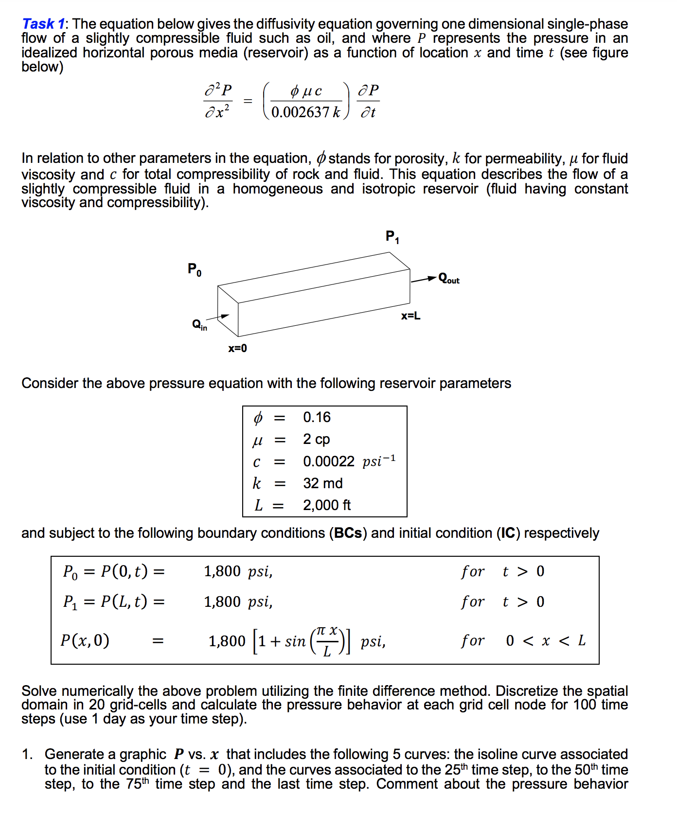
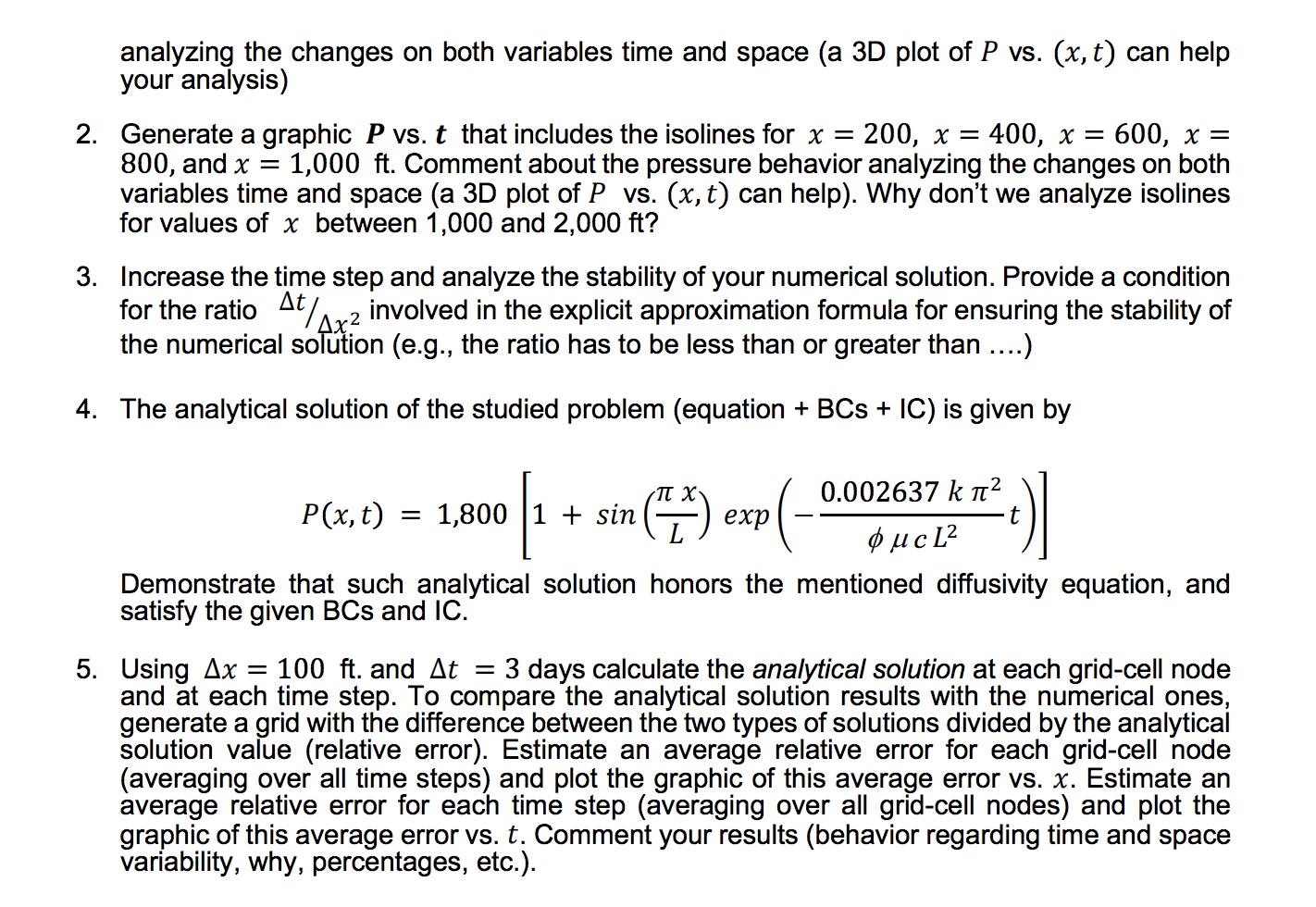
Task 1: The equation below gives the diffusivity equation governing one dimensional single-phase ow of a slightly compressible fluid such as oil, and where P represents the pressure in an idealized horizontal porous media (reservoir) as a function of location x and time it (see figure below) azp _ [ gripe J 5x2 0.0026371: 't In relation to other parameters in the equation, stands for porosity, k for permeability, p for fluid viscosity and c for total compressibility of rock and uid. This equation describes the ow of a slightlyty co mJJressible uid in a homogeneous and isotropic reservoir (uid having constant viscosity an compressibility). 0.16 2 cp 0.00022 psi1 32 md 2,000 ft and subject to the following boundary conditions (865) and initial condition (IC) respectively P0 = P(0, t) = 1,800 psi, P1 = P(L, t) = 1,800 psi, P(x, 0) 1 800 [1 + sin (ELx\" psi, Solve numerically the above problem utilizing the nite difference method. Discretize the spatial domain in 20 grid-cells and calculate the pressure behavior at each grid cell node for 100 time steps (use 1 day as your time step). 1. Generate a graphic P vs. at that includes the following 5 curves: the isoline curve associated to the initial condition (t = 0), and the curves associated to the 25th time step, to the 50111 time step, to the 75111 time step and the last time step. Comment about the pressure behavior analyzing the changes on both variables time and space (a 3D plot of P vs. (x, t) can help your analysis) . Generate a graphic P vs. t that includes the isolines for x = 200, x = 400, x = 600, x = 800, and x = 1,000 ft. Comment about the pressure behavior analyzing the changes on both variables time and space (a 3D plot of P vs. (x, t) can help). Why don't we analyze isolines for values of at between 1,000 and 2,000 ft? . Increase the time step and analyze the stability of your numerical solution. Provide a condition for the ratio 33/ 2 involved in the explicit approximation formula for ensuring the stability of the numerical soion (e.g., the ratio has to be less than or greater than ....) . The analytical solution of the studied problem (equation + BCs + IC) is given by _ nx 0.002637 kHz 1 + sm() exp t L We? Demonstrate that such analytical solution honors the mentioned diffusivity equation, and satisfy the given BCs and IC. P(x, t) = 1,800 Using Ax = 100 ft. and At = 3 days calculate the analytical solution at each grid-cell node and at each time step. To compare the analytical solution results with the numerical ones, generate a grid with the difference between the two types of solutions divided by the analytical solution value (relative error). Estimate an average relative error for each grid-cell node (averaging over all time steps) and plot the graphic of this average error vs. x. Estimate an average relative error for each time step (averaging over all grid-cell nodes) and plot the graphic of this average error vs. t. Comment your results (behavior regarding time and space variability, why, percentages, etc.)