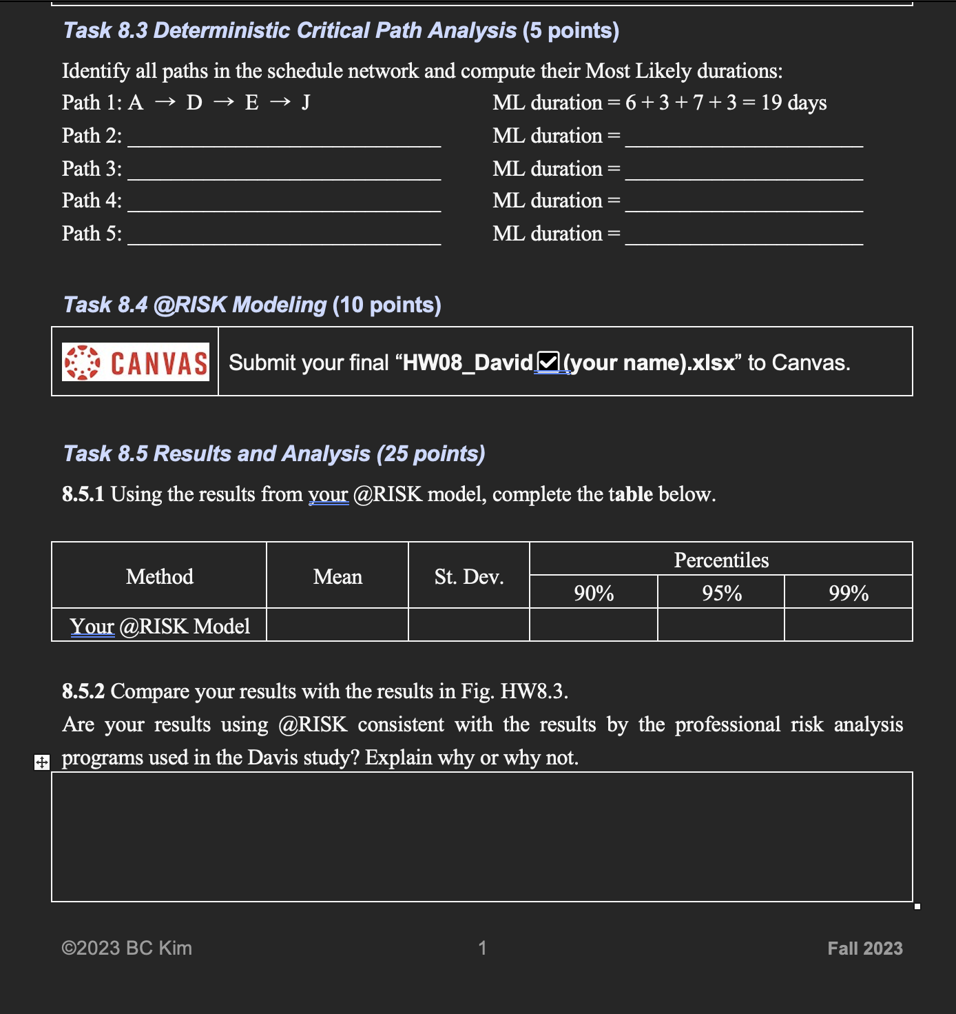
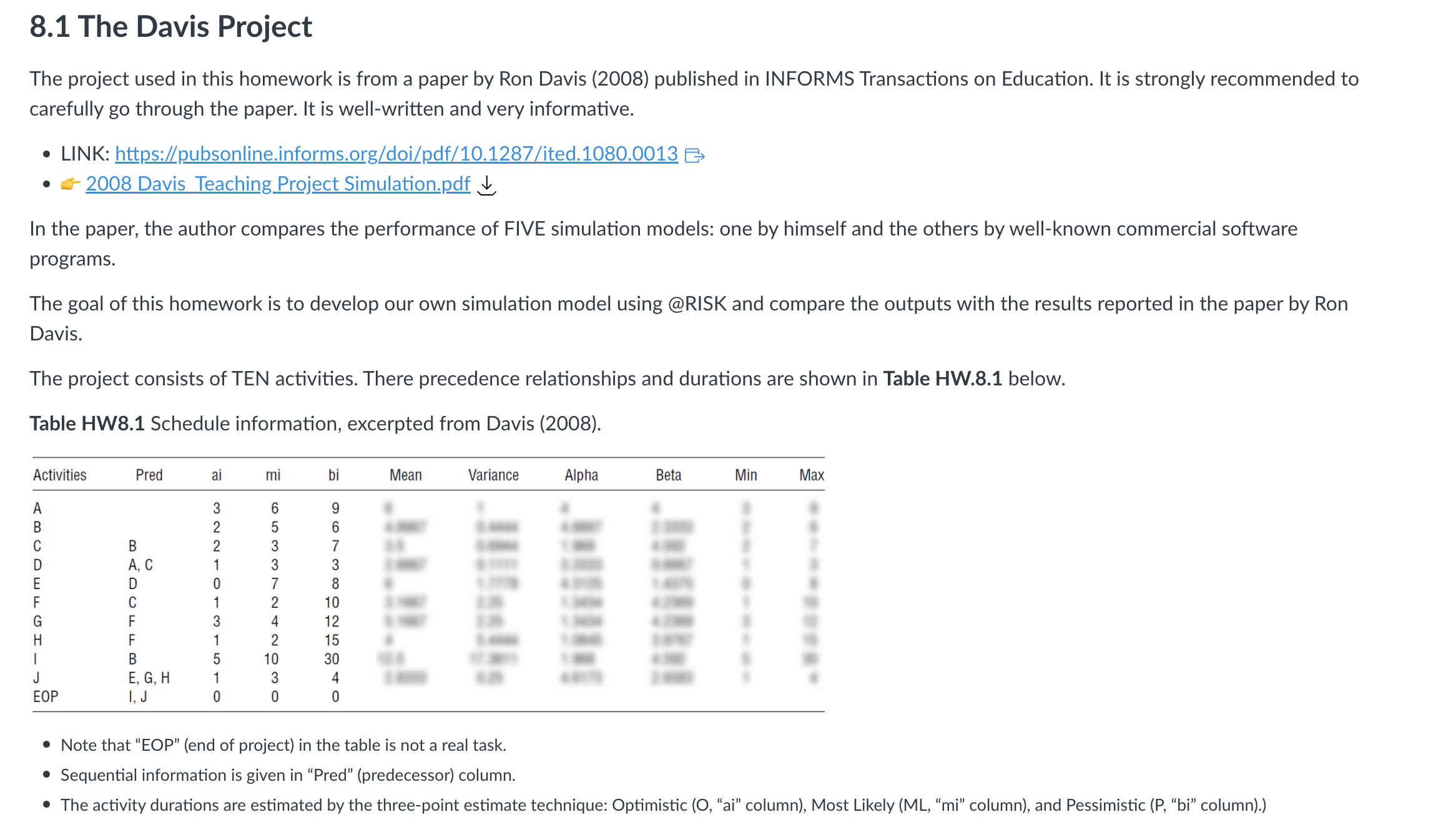
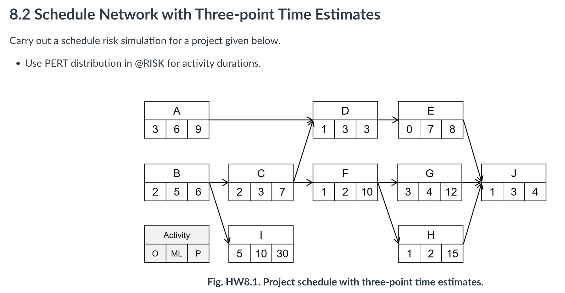
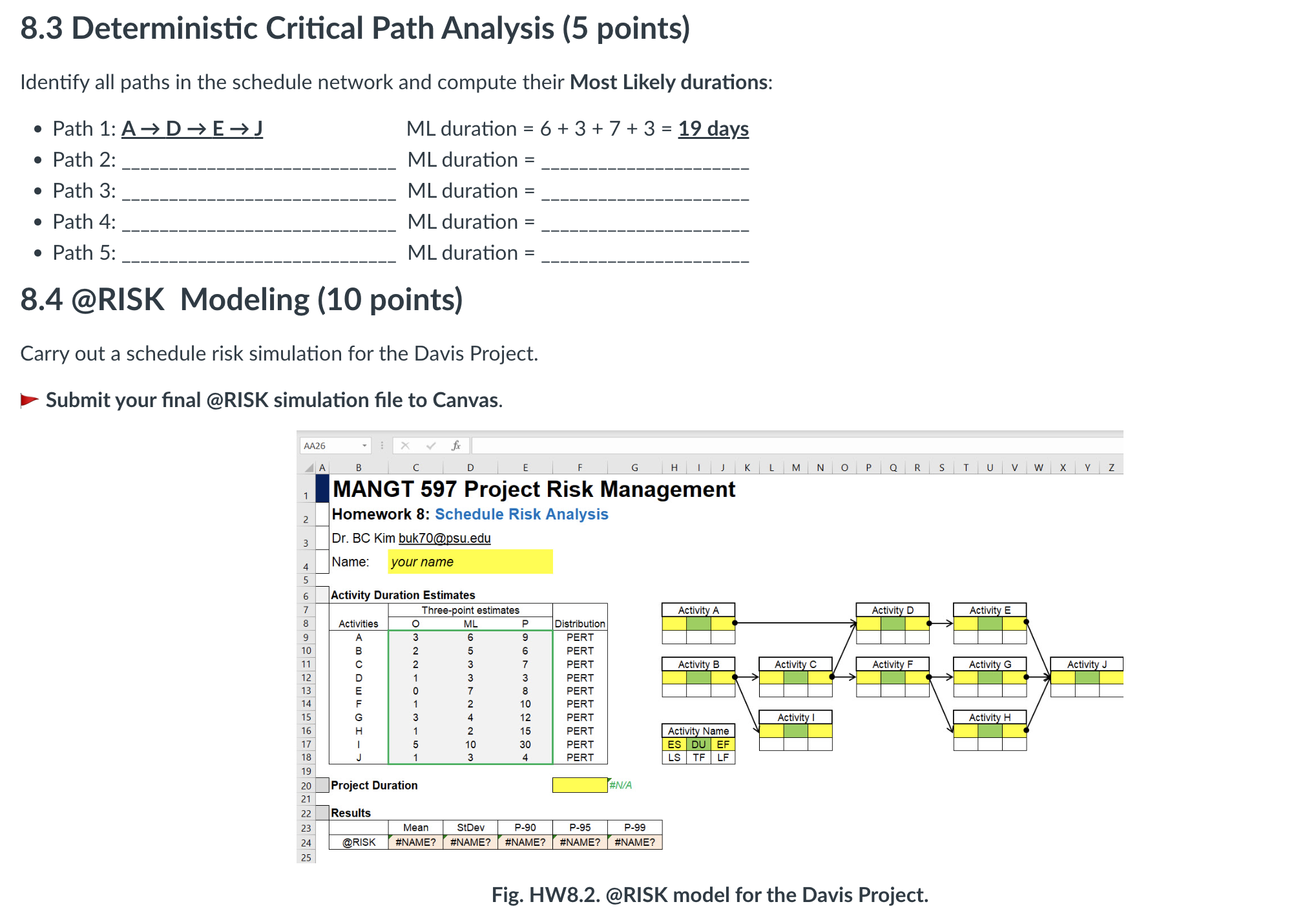
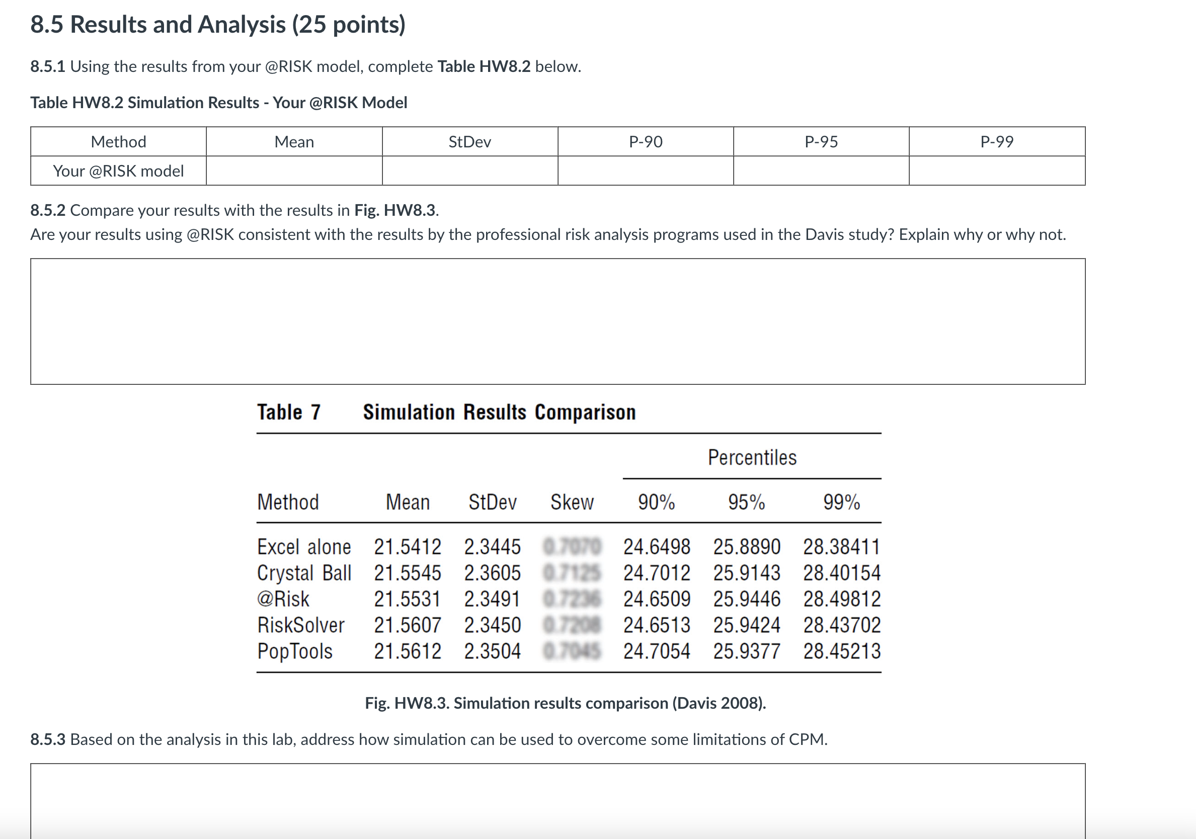
Task 8.3 Deterministic Critical Path Analysis (5 points) Identify all paths in the schedule network and compute their Most Likely durations: Path 1: A - D - E - J ML duration = 6+3+7+ 3 = 19 days Path 2: ML duration = Path 3: ML duration = Path 4: ML duration = Path 5: ML duration = Task 8.4 @RISK Modeling (10 points) CANVAS |Submit your final "HW08_David (your name).xisx" to Canvas. Task 8.5 Results and Analysis (25 points) 8.5.1 Using the results from your @RISK model, complete the table below. Percentiles Method Mean St. Dev. 90% 95% 99% Your @RISK Model 8.5.2 Compare your results with the results in Fig. HW8.3. Are your results using @RISK consistent with the results by the professional risk analysis + programs used in the Davis study? Explain why or why not. 2023 BC Kim Fall 20238.1 The Davis Project The project used in this homework is from a paper by Ron Davis (2008) published in INFORMS Transactions on Education. It is strongly recommended to carefully go through the paper. It is well-written and very informative. . LINK: https://pubsonline.informs.org/doi/pdf/10.1287/ited. 1080.0013 => . 2008 Davis Teaching Project Simulation.pdf In the paper, the author compares the performance of FIVE simulation models: one by himself and the others by well-known commercial software programs. The goal of this homework is to develop our own simulation model using @RISK and compare the outputs with the results reported in the paper by Ron Davis. The project consists of TEN activities. There precedence relationships and durations are shown in Table HW.8.1 below. Table HW8.1 Schedule information, excerpted from Davis (2008). Activities Pred ai mi bi Mean Variance Alpha Beta Min Max O - N NW A, C - -IS TMOOOD 100 O W O N D N V WWOD - 01 - W E, G, H EOP 1, J Note that "EOP" (end of project) in the table is not a real task. . Sequential information is given in "Pred" (predecessor) column. . The activity durations are estimated by the three-point estimate technique: Optimistic (O, "ai" column), Most Likely (ML, "mi" column), and Pessimistic (P, "bi" column).)8.2 Schedule Network with Three-point Time Estimates Carry out a schedule risk simulation for a project given below. . Use PERT distribution in @RISK for activity durations. A D F 3 6 9 1 3 3 0 7 8 B C F G C 2 5 6 2 3 7 1 2 10 3 4 12 1 3 4 Activity H O ML P 5 10 30 1 2 15 Fig. HW8.1. Project schedule with three-point time estimates.8.3 Deterministic Critical Path Analysis (5 points) Identify all paths in the schedule network and compute their Most Likely durations: . Path 1: A -> D - E-> J ML duration = 6 + 3 +7 + 3 = 19 days . Path 2: ML duration = . Path 3: ML duration = . Path 4: ML duration = . Path 5: ML duration = 8.4 @RISK Modeling (10 points) Carry out a schedule risk simulation for the Davis Project. Submit your final @RISK simulation file to Canvas. AA26 1 X A B D G H I J K L M N O P Q R S T U V W X Y Z MANGT 597 Project Risk Management Homework 8: Schedule Risk Analysis N 3 Dr. BC Kim buk70@psu.edu Name: your name Activity Duration Estimates D CO V MI VIA Three-point estimates Activity A Activity D Activity E Activities ML P Distribution PERT 10 PERT 11 PERT ACTIVITY BY Activity C Activity F ACTIVITY G Activity J 12 PERT 13 -U - W - O - N N W O PERT 14 PERT 15 4 PER Activity | Activity H 16 2 PERT Activity Name 17 10 PERT ES DU EF 18 2 A PERT LS TF |LF 19 20 Project Duration #N/A 22 Results 23 Mean StDev P-90 P-95 P-99 24 @RISK #NAME? #NAME? #NAME? #NAME? #NAME? 25 Fig. HW8.2. @RISK model for the Davis Project.8.5 Results and Analysis (25 points) 8.5.1 Using the results from your @RISK model, complete Table HW8.2 below. Table HW8.2 Simulation Results - Your @RISK Model Method Mean StDev P-90 P-95 P-99 Your @RISK model 8.5.2 Compare your results with the results in Fig. HW8.3. Are your results using @RISK consistent with the results by the professional risk analysis programs used in the Davis study? Explain why or why not. Table 7 Simulation Results Comparison Percentiles Method Mean StDev Skew 90% 95% 99% Excel alone 21.5412 2.3445 0.7070 24.6498 25.8890 28.38411 Crystal Ball 21.5545 2.3605 0.7125 24.7012 25.9143 28.40154 @Risk 21.5531 2.3491 0.7236 24.6509 25.9446 28.49812 RiskSolver 21.5607 2.3450 0.7208 24.6513 25.9424 28.43702 Pop Tools 21.5612 2.3504 0.7045 24.7054 25.9377 28.45213 Fig. HW8.3. Simulation results comparison (Davis 2008). 8.5.3 Based on the analysis in this lab, address how simulation can be used to overcome some limitations of CPM.8.5.3 Based on the analysis in this lab, address how simulation can be used to overcome some limitations of CPM