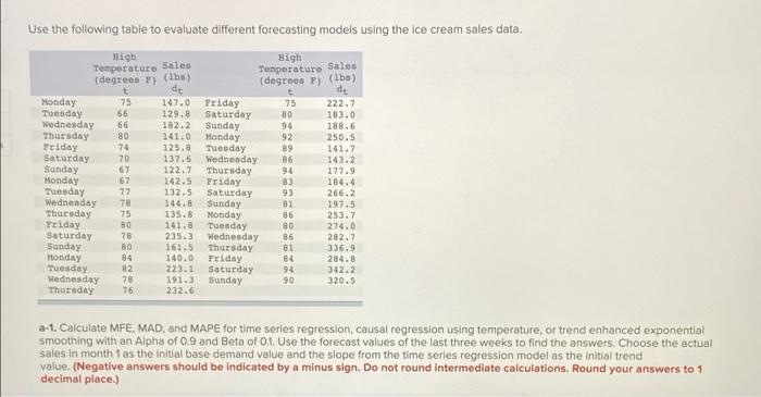
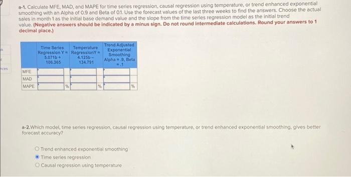
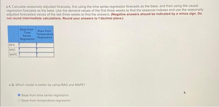
Temperature Sales Use the following table to evaluate different forecasting models using the ice cream sales data. High High Temperature Sales (degrees F) (lbs) (degrees P) (lbs) de t de Monday 75 147.0 Priday 75 222.7 Tuesday 66 129.8 Saturday 80 183.0 Wednesday 66 182.2 Sunday 94 188.6 Thursday BO 141.0 Monday 92 250.5 Friday 74 125.8 Tuesday 89 141.7 Saturday 70 137.6 Wedne day 86 143.2 Sunday 67 122.2 Thursday 94 177.9 Monday 67 142.5 Friday 184.4 Tuesday 77 132.5 Saturday 93 266.2 Wednenday 78 144.8 Sunday 81 197.5 Thursday 75 135.8 Monday 86 253.7 Friday 80 141.8 Tuesday 80 274.0 Saturday 28 235.3 Wednesday 86 282.7 Sunday 80 161.5 Thursday 81 336.9 Monday 84 140.0 Priday B4 284.8 Tuesday 82 223.1 Saturday 94 342.2 Wednesday 78 191.3 Sunday 90 320.5 Thursday 76 232.6 a-1. Calculate MFE. MAD, and MAPE for time series regression, causal regression using temperature, or trend enhanced exponential smoothing with an Alpha of 0.9 and Beta of 0.1. Use the forecast values of the last three weeks to find the answers. Choose the actual sales in month 1 as the initial base demand value and the slope from the time series regression model as the initial trend value. (Negative answers should be indicated by a minus sign. Do not round intermediate calculations. Round your answers to 1 decimal place.) 6-1. Calculate MFE. MAD, and MAPE for time series regression, causal regression using temperature, or trend enhanced exponential smoothing with an Alpha of 0.9 and Beta of 0.1. Use the forecast values of the last three weeks to find the answers. Choose the actual sales in month as the initial base demand value and the slope from the time series regression model as the initial trend value. (Negative answers should be indicated by a minus sign. Do not round intermediate calculations. Round your answers to 1 decimal place.) Time Series Temperature Regression Y = Rogression Y = 5.071b- 4.125 106.365 134,791 Trend Adjusted Exponential Smoothing Alpha 9, Bota 2.1 MFE MAD MAPE a-2.Which model, time series regression, causal regression using temperature, or trend enhanced exponential smoothing, gives better forecast accuracy? Trend enhanced exponential smoothing Time series regression Cousal regression using temperature C-1. Calculate seasonally adjusted forecasts, first using the time series regression forecasts as the base, and then using the causal regression forecasts as the base. Use the demand values of the first three weeks to find the seasonal indexes and use the seasonally adjusted forecasted values of the last three weeks to find the answers. (Negative answers should be indicated by a minus sign. Do not round intermediate calculations. Round your answers to 1 decimal place.) Base from Time Series Base from Temperature Regression Repression MFE MAD MAPE c-2. Which modelis better by using MAD and MAPE? Base from time series regression Base from temperature regression Temperature Sales Use the following table to evaluate different forecasting models using the ice cream sales data. High High Temperature Sales (degrees F) (lbs) (degrees P) (lbs) de t de Monday 75 147.0 Priday 75 222.7 Tuesday 66 129.8 Saturday 80 183.0 Wednesday 66 182.2 Sunday 94 188.6 Thursday BO 141.0 Monday 92 250.5 Friday 74 125.8 Tuesday 89 141.7 Saturday 70 137.6 Wedne day 86 143.2 Sunday 67 122.2 Thursday 94 177.9 Monday 67 142.5 Friday 184.4 Tuesday 77 132.5 Saturday 93 266.2 Wednenday 78 144.8 Sunday 81 197.5 Thursday 75 135.8 Monday 86 253.7 Friday 80 141.8 Tuesday 80 274.0 Saturday 28 235.3 Wednesday 86 282.7 Sunday 80 161.5 Thursday 81 336.9 Monday 84 140.0 Priday B4 284.8 Tuesday 82 223.1 Saturday 94 342.2 Wednesday 78 191.3 Sunday 90 320.5 Thursday 76 232.6 a-1. Calculate MFE. MAD, and MAPE for time series regression, causal regression using temperature, or trend enhanced exponential smoothing with an Alpha of 0.9 and Beta of 0.1. Use the forecast values of the last three weeks to find the answers. Choose the actual sales in month 1 as the initial base demand value and the slope from the time series regression model as the initial trend value. (Negative answers should be indicated by a minus sign. Do not round intermediate calculations. Round your answers to 1 decimal place.) 6-1. Calculate MFE. MAD, and MAPE for time series regression, causal regression using temperature, or trend enhanced exponential smoothing with an Alpha of 0.9 and Beta of 0.1. Use the forecast values of the last three weeks to find the answers. Choose the actual sales in month as the initial base demand value and the slope from the time series regression model as the initial trend value. (Negative answers should be indicated by a minus sign. Do not round intermediate calculations. Round your answers to 1 decimal place.) Time Series Temperature Regression Y = Rogression Y = 5.071b- 4.125 106.365 134,791 Trend Adjusted Exponential Smoothing Alpha 9, Bota 2.1 MFE MAD MAPE a-2.Which model, time series regression, causal regression using temperature, or trend enhanced exponential smoothing, gives better forecast accuracy? Trend enhanced exponential smoothing Time series regression Cousal regression using temperature C-1. Calculate seasonally adjusted forecasts, first using the time series regression forecasts as the base, and then using the causal regression forecasts as the base. Use the demand values of the first three weeks to find the seasonal indexes and use the seasonally adjusted forecasted values of the last three weeks to find the answers. (Negative answers should be indicated by a minus sign. Do not round intermediate calculations. Round your answers to 1 decimal place.) Base from Time Series Base from Temperature Regression Repression MFE MAD MAPE c-2. Which modelis better by using MAD and MAPE? Base from time series regression Base from temperature regression