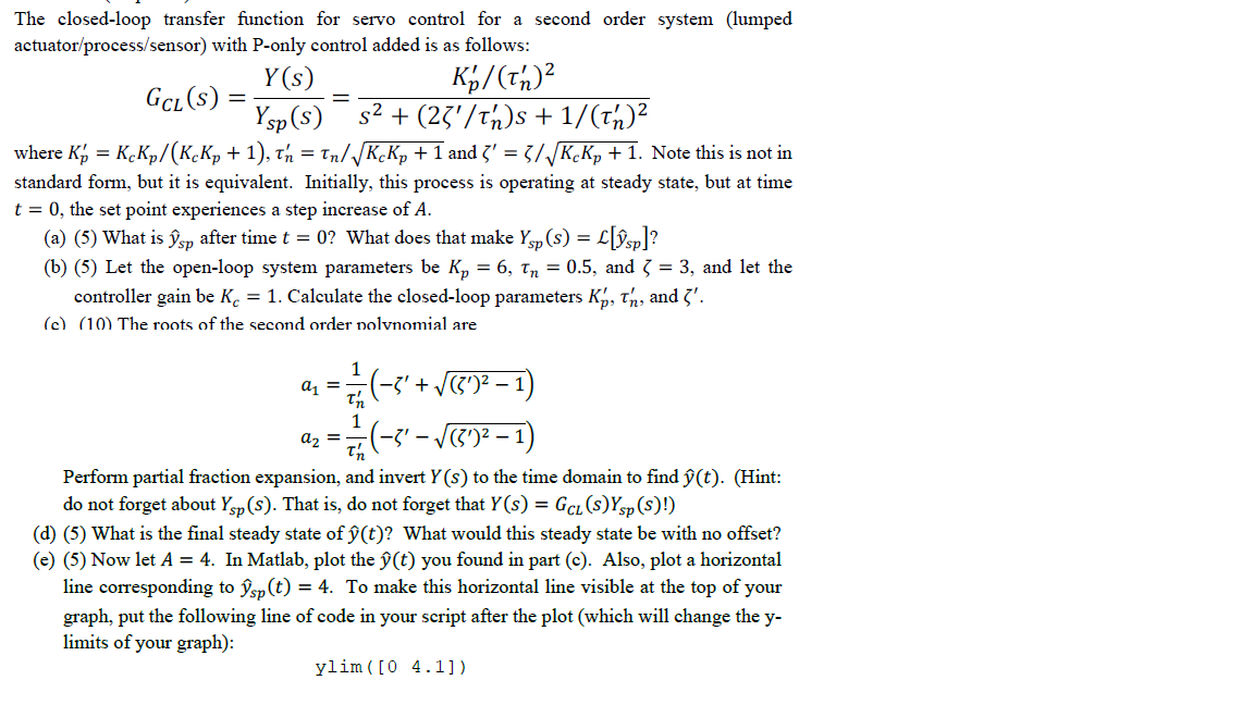
The closed-loop transfer function for servo control for a second order system (lumped actuator/process/sensor) with P-only control added is as follows: GCL(s)=Ysp(s)Y(s)=s2+(2)s+1/(n)2Kp/(n)2 where Kp=KcKp/(KcKp+1),n=n/KcKp+1 and =/KcKp+1. Note this is not in standard form, but it is equivalent. Initially, this process is operating at steady state, but at time t=0, the set point experiences a step increase of A. (a) (5) What is y^sp after time t=0 ? What does that make Ysp(s)=L[y^sp] ? (b) (5) Let the open-loop system parameters be Kp=6,n=0.5, and =3, and let the controller gain be Kc=1. Calculate the closed-loop parameters Kp,n, and . (c) (10) The roots of the second order nolvnomial are a1=n1(+()21)a2=n1(()21) Perform partial fraction expansion, and invert Y(s) to the time domain to find y^(t). (Hint: do not forget about Ysp(s). That is, do not forget that Y(s)=GCL(s)Ysp(s)!) (d) (5) What is the final steady state of y^(t) ? What would this steady state be with no offset? (e) (5) Now let A=4. In Matlab, plot the y^(t) you found in part (c). Also, plot a horizontal line corresponding to y^sp(t)=4. To make this horizontal line visible at the top of your graph, put the following line of code in your script after the plot (which will change the y limits of your graph): ylim([04.1])