The MAD for Method 1=______thousands gallons (round your response to three decimal places)

The mean squared error (MSE) for Method 1=______thousands gallons^2(round your response to three decimal places)

The MAD for method 2=____thousands gallons (round your response to three decimal places)

The mean squared error (MSE) for Method 2=____thousands gallons^2 (round your response to three decimal places)

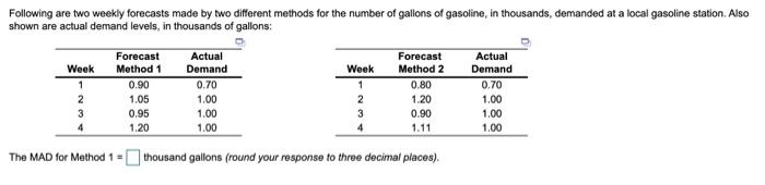
Following are two weekly forecasts made by two different methods for the number of gallons of gasoline, in thousands, demanded at a local gasoline station. Also shown are actual demand levels, in thousands of gallons Week 1 2 3 4 Forecast Method 1 0.90 1.05 0.95 1.20 Actual Demand 0.70 1.00 1.00 1.00 Week 1 2 3 4 Forecast Method 2 0.80 1.20 0.90 1.11 Actual Demand 0.70 1.00 1.00 1.00 The MAD for Method 1 = thousand gallons (round your response to three decimal places). Mark Gershon, owner of a musical instrument distributorship, thinks that demand for guitars may be related to the number of television appearances by the popular group Maroon 5 during the previous month. Gershon has collected the data shown in the following table: Maroon 5 TV Appearances 3 3 8 5 8 7 Demand for Guitars 3 6 7 5 11 8 This exercise contains only parts b, c, and d. b) Using the least squares regression method, the equation for forecasting is (round your responses to four decimal places): Y. 1.4146 . 0.9268 c) The estimato for guitar sales i Maroon 5 performed on TV 11 times - 11.61 sales (round your response to two decimal places). d) The correlation coefficient (1) for this model = 0.7938 (round your response to four decimal places), The coefficient of determination () for this model =(round your response to four docimal places), Bus and subway ridership for the summer months in London, England, is believed to be tied heavily to the number of tourists visiting the city. During the past 12 years, the following data have been obtained: 1 7 1.5 2 2 1.1 3 6 1.4 4 4 1.5 5 14 2.4 6 15 2.7 7 16 2.4 8 12 1.9 9 14 2.6 10 20 4.4 11 15 3.4 12 7 1.7 Year Number of Tourists (in millions) Ridership (in millions) This exercise contains only parts b, c, d, e, and 1. b) The least-squares regression equation that shows the best relationship between ridership and the number of tourists is (round your responses to three decimal places): - 0.665 + 0.153 x where y = Dependent Variable and x = Independent Variable c) If it is expected that 10 million tourists will visit London, then the expected ridership = 2.10 million riders (round your response to two decimal places). d) If there are no tourists at all, then the model still predicts a ridership. This is due to the fact that zero tourists are outside the range of data used to develop the model. 6) The standard error of the estimate developed using least-squares regression fround your response to three places)