

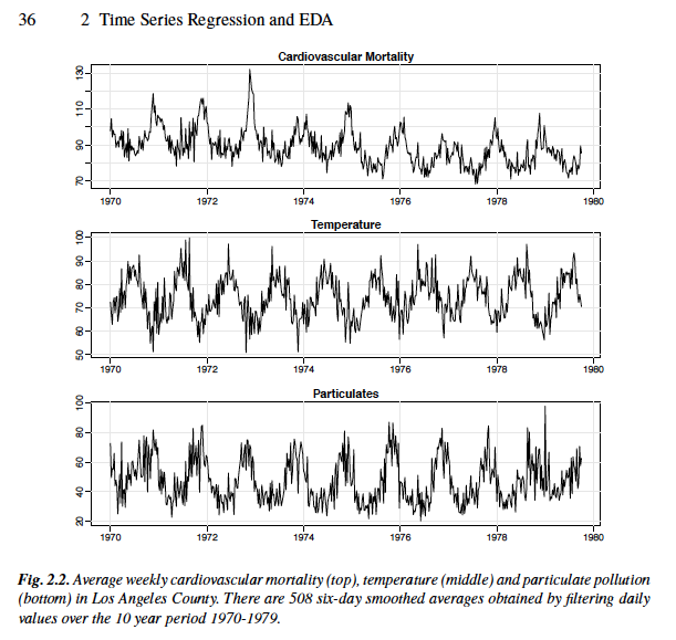
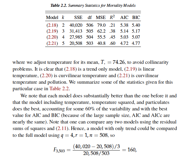
Question: The R CODE of loading data packages: install.packages(astsa) library(astsa) par(mfrow=c(3,1)) # plot the data tsplot(cmort, main=Cardiovascular Mortality, ylab=) tsplot(tempr, main=Temperature, ylab=) tsplot(part, main=Particulates, ylab=) dev.new()

The R CODE of loading data packages:
install.packages("astsa")
library(astsa)
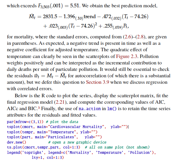
par(mfrow=c(3,1)) # plot the data
tsplot(cmort, main="Cardiovascular Mortality", ylab="")
tsplot(tempr, main="Temperature", ylab="")
tsplot(part, main="Particulates", ylab="")
dev.new() # open a new graphic device
ts.plot(cmort,tempr,part, col=1:3) # all on same plot (not shown)
legend('topright', legend=c('Mortality', 'Temperature', 'Pollution'),
lty=1, col=1:3)
dev.new()
pairs(cbind(Mortality=cmort, Temperature=tempr, Particulates=part))
temp = tempr-mean(tempr) # center temperature
temp2 = temp^2
trend = time(cmort) # time
fit = lm(cmort~ trend + temp + temp2 + part, na.action=NULL)
summary(fit) # regression results
summary(aov(fit)) # ANOVA table (compare to next line)
summary(aov(lm(cmort~cbind(trend, temp, temp2, part)))) # Table 2.1
num = length(cmort) # sample size
AIC(fit)um - log(2*pi) # AIC
BIC(fit)um - log(2*pi) # BIC
(AICc = log(sum(resid(fit)^2)um) + (num+5)/(num-5-2)) # AICc
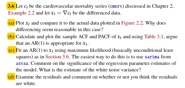
ct ct be the cardiovascular mortality series (ort) discussed in Chapter 2, Example 2.2 and let Xt Ct be the differenced data. Plot x and compare it to the actual data plotted in Figure 2.2. Why does differencing seem reasonable in this case? that an AR(1) is appropriate for x squares) as in Section 3.6. The easiest way to do this is to use sarima from the model. What is t (b) Calculate and plot the sample ACF and PACF of x and using Table 3.1, argue (c) Fit an AR(1) to Xt using maximum likelihood (basically unconditional least he estimate of the whiten (d) Examine the residuals and comment on whether or not you think the residuals are white. ct ct be the cardiovascular mortality series (ort) discussed in Chapter 2, Example 2.2 and let Xt Ct be the differenced data. Plot x and compare it to the actual data plotted in Figure 2.2. Why does differencing seem reasonable in this case? that an AR(1) is appropriate for x squares) as in Section 3.6. The easiest way to do this is to use sarima from the model. What is t (b) Calculate and plot the sample ACF and PACF of x and using Table 3.1, argue (c) Fit an AR(1) to Xt using maximum likelihood (basically unconditional least he estimate of the whiten (d) Examine the residuals and comment on whether or not you think the residuals are white
Step by Step Solution
There are 3 Steps involved in it

Get step-by-step solutions from verified subject matter experts