The R&D group of a major public utility company has identified eight possible projects. A net present value analysis has computed: (1) the expected revenue for each project if it is successful, (2) the estimated probability of success for each project, and (3) the initial investment required for each project. Using these figures, the finance manager has computed the expected return and the expected profit for each project as shown in the Model worksheet. Unfortunately, the available budget is only $2.0 million, and selecting all projects would require a total initial investment of $2.8 million. Thus, the problem is to determine which projects to select to maximize the total expected profit while staying within the budget limitation. Complicating this decision is the fact that both the expected revenue and success rates are highly uncertain.

Each of the eight projects has an Expected Revenue and Success Rate. The product of those two factors equals the Expected Return, and the Expected Profit is the Expected Return less the Initial Investment for a selected project. The decisions in Column H are binary; that is, they can assume only the values zero and one, representing the decisions of either not selecting or selecting each project. With a one (a "go" decision), the project's Expected Profit is calculated. With a zero (a "no-go" decision), the Expected profit becomes zero. The Investment in cell F15 is the required investment in column F multiplied by the respective decision variable in column H.

The expected revenue and success rates are uncertain, and although good solutions might be identified by inspection or by trial and error, basing a decision on expected values can be dangerous because it doesn’t assess the risks. In reality, selecting R&D projects is a one-time decision; each project will be either successful or not. If a project is not successful, the company runs the risk of incurring the loss of the initial investment. Thus, incorporating risk analysis within the context of the optimization is a very useful approach.

The assumptions for revenues are the following:

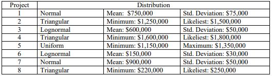
The other eight assumptions represent the success rates for each project. These rates are modeled using a binomial distribution with one trial.

The forecast variable is Total Profit.

The eight decision variables defined in this model are in Column H, and as described before, these will be either a one or a zero.

Project	Expected Revenue	Success Rate	Expected Return	Initial Investment	Expected Profit	Decisions
1	$        750,000	90%	$            675,000	$            250,000	$            425,000	1
2	$    1,500,000	70%	$        1,050,000	$            650,000	$            400,000	1
3	$        600,000	60%	$            360,000	$            250,000	$            110,000	1
4	$    1,800,000	40%	$            720,000	$            500,000	$            220,000	1
5	$    1,250,000	80%	$        1,000,000	$            700,000	$            300,000	1
6	$        150,000	60%	$              90,000	$              30,000	$              60,000	1
7	$        900,000	70%	$            630,000	$            350,000	$            280,000	1
8	$        250,000	90%	$            225,000	$              70,000	$            155,000	1
			Budget	$        2,000,000
			Invested	$        2,800,000
			Surplus	($800,000)

Total profit

$        1,950,000

Maximize total expected profit subject to budget constraint.

Use Crystal Ball and show the complete solution.

 

Transcribed Image Text:

Project I 2 3 4 5 6 7 8 Normal Triangular Lognormal Triangular Uniform Lognormal Normal Triangular Distribution Mean: $750,000 Minimum: $1,250,000 Mean: $600,000 Minimum: $1,600,000 Minimum: $1,150,000 Mean: $150,000 Mean: $900,000 Minimum: $220,000 Std. Deviation: $75,000 Likeliest: $1,500,000 Std. Deviation: $50,000 Likeliest: $1,800,000 Maximum: $1,350,000 Std. Deviation: $30,000 Std. Deviation: $50,000 Likeliest: $250,000 Project I 2 3 4 5 6 7 8 Normal Triangular Lognormal Triangular Uniform Lognormal Normal Triangular Distribution Mean: $750,000 Minimum: $1,250,000 Mean: $600,000 Minimum: $1,600,000 Minimum: $1,150,000 Mean: $150,000 Mean: $900,000 Minimum: $220,000 Std. Deviation: $75,000 Likeliest: $1,500,000 Std. Deviation: $50,000 Likeliest: $1,800,000 Maximum: $1,350,000 Std. Deviation: $30,000 Std. Deviation: $50,000 Likeliest: $250,000

Answer rating: 100% (QA)

The expected revenue and success rates are assumptio... View the full answer