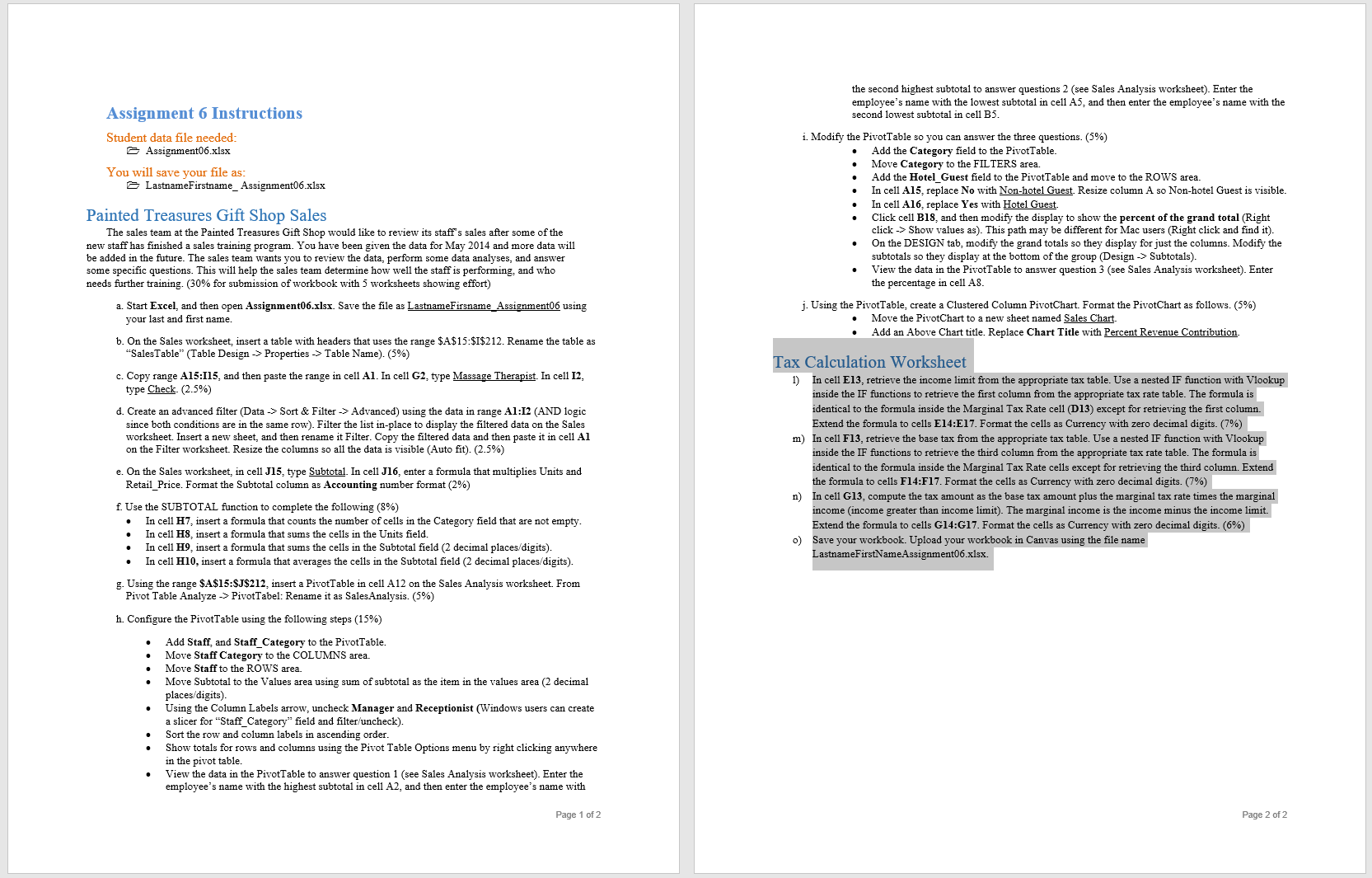
the second highest subtotal to answer questions 2 (see Sales Analysis worksheet). Enter the employee's name with the lowest subtotal in cell AS, and then enter the employee's name with the Assignment 6 Instructions second lowest subtotal in cell B5. Student data file needed: i. Modify the PivotTable so you can answer the three questions. (5%) Assignment06.xlex . Add the Category field to the PivotTable. Move Category to the FILTERS area. You will save your file as: . Add the Hotel_Guest field to the PivotTable and move to the ROWS area. LastnameFirstname_ Assignment06.xlex . In cell A15, replace No with Non-hotel Guest. Resize column A so Non-hotel Guest is visible. In cell A16, replace Yes with Hotel Guest. Painted Treasures Gift Shop Sales Click cell B18, and then modify the display to show the percent of the grand total (Right The sales team at the Painted Treasures Gift Shop would like to review its staff's sales after some of the click -> Show values as). This path may be different for Mac users (Right click and find it). new staff has finished a sales training program. You have been given the data for May 2014 and more data will . On the DESIGN tab, modify the grand totals so they display for just the columns. Modify the be added in the future. The sales team wants you to review the data, perform some data analyses, and answer subtotals so they display at the bottom of the group (Design -> Subtotals) some specific questions. This will help the sales team determine how well the staff is performing, and who View the data in the PivotTable to answer question 3 (see Sales Analysis worksheet). Enter needs further training. (30% for submission of workbook with 5 worksheets showing effort) the percentage in cell AS a. Start Excel, and then open Assignment06.xIsx. Save the file as LastnameFirsname_Assignment06 using j. Using the PivotTable, create a Clustered Column PivotChart. Format the PivotChart as follows. (5%) your last and first name. Move the PivotChart to a new sheet named Sales Chart Add an Above Chart title. Replace Chart Title with Percent Revenue Contribution. b. On the Sales worksheet, insert a table with headers that uses the range $A$15:$1$212. Rename the table as "SalesTable" (Table Design -> Properties -> Table Name). (5%) Tax Calculation Worksheet c. Copy range A15:115, and then paste the range in cell Al. In cell G2, type Massage Therapist. In cell 12, 1) In cell E13, retrieve the income limit from the appropriate tax table. Use a nested IF function with Vlookup type Check. (2.5%) inside the IF functions to retrieve the first column from the appropriate tax rate table. The formula is d. Create an advanced filter (Data -> Sort & Filter -> Advanced) using the data in range A1:12 (AND logic identical to the formula inside the Marginal Tax Rate cell (D13) except for retrieving the first column. since both conditions are in the same row). Filter the list in-place to display the filtered data on the Sales Extend the formula to cells E14:E17. Format the cells as Currency with zero decimal digits. (7%) worksheet. Insert a new sheet, and then rename it Filter. Copy the filtered data and then paste it in cell Al m) In cell F13, retrieve the base tax from the appropriate tax table. Use a nested IF function with Vlookup on the Filter worksheet. Resize the columns so all the data is visible (Auto fit). (2.5%) inside the IF functions to retrieve the third column from the appropriate tax rate table. The formula is e. On the Sales worksheet, in cell J15, type Subtotal. In cell J16, enter a formula that multiplies Units and identical to the formula inside the Marginal Tax Rate cells except for retrieving the third column. Extend Retail Price. Format the Subtotal column as Accounting number format (2%) the formula to cells F14:F17. Format the cells as Currency with zero decimal digits. (7%) In cell G13, compute the tax amount as the base tax amount plus the marginal tax rate times the marginal . Use the SUBTOTAL function to complete the following (8%) income (income greater than income limit). The marginal income is the income minus the income limit. In cell H7, insert a formula that counts the number of cells in the Category field that are not empty. Extend the formula to cells G14:G17. Format the cells as Currency with zero decimal digits. (6%) In cell H8, insert a formula that sums the cells in the Units field. In cell H9, insert a formula that sums the cells in the Subtotal field (2 decimal places/digits). Save your workbook. Upload your workbook in Canvas using the file name In cell H10, insert a formula that averages the cells in the Subtotal field (2 decimal places/digits). LastnameFirstNameAssignment06.xlex. g. Using the range $A$15:$J$212, insert a PivotTable in cell A12 on the Sales Analysis worksheet. From Pivot Table Analyze -> PivotTabel: Rename it as SalesAnalysis. (5%) h. Configure the PivotTable using the following steps (15%) Add Staff, and Staff_Category to the PivotTable. Move Staff Category to the COLUMNS area. Move Staff to the ROWS area. Move Subtotal to the Values area using sum of subtotal as the item in the values area (2 decimal places/digits). Using the Column Labels arrow, uncheck Manager and Receptionist (Windows users can create a slicer for "Staff_Category" field and filter/uncheck) Sort the row and column labels in ascending order. Show totals for rows and columns using the Pivot Table Options menu by right clicking anywhere in the pivot table. View the data in the PivotTable to answer question 1 (see Sales Analysis worksheet). Enter the employee's name with the highest subtotal in cell A2, and then enter the employee's name with Page 1 of 2 Page 2 of 2