This example builds on the electronics superstore and warehouse examples, by considering them simultaneously in a multi-level supply chain. Thus, the store management now has control of two levels of the supply chain. The key question is still: How much and when to order? However, management now must consider inventory that occurs in several places of the process, including the delivery trucks!

Consider a company that manages two electronics stores that sell the same popular handheld computer. Orders are placed to a regional warehouse, also owned by this company. The regional warehouse places orders to the manufacturer (which is not owned by the company). The amount of time to receive an order at either store can be approximated by a normal distribution with a mean of 1 day and a standard deviation of .1 days. The amount of time to receive an order at the warehouse can be approximated by a normal distribution, with a mean of 4 days and a standard deviation of .2 days. The mean demand for this computer at each store is five computers per day (both stores are open 10 hours per day, 7 days per week). The demand is expected to remain the same at both stores for the next 60 days.

Management wants to use a reorder point scheme at the stores and the warehouse. Their goal is to achieve at least a 95% service level at each store at minimum cost. The ordering costs are $75 every time a store places an order to the warehouse and $150 every time the warehouse places an order to the factory. It also costs $.50 per day for every computer in inventory at a store, and $.10 per day for every computer in inventory at the warehouse. We assume it also costs $.10 per day for every computer in transit from the warehouse to a store.

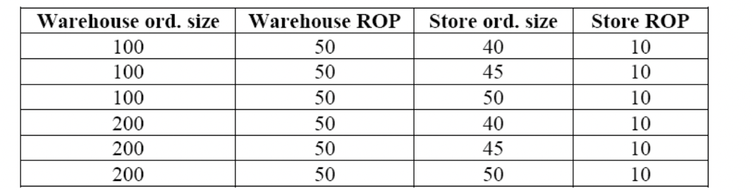
Build the SimQuick model. For each scenario (row) in the following table, run 40 simulations and report the mean of the overall mean service levels for the two stores and the estimated total cost. Which scenario should management adopt?

Note: Although it may not seem obvious at first, this example is a special case of the just-intime (JIT) system typically used in manufacturing to control the flow of inventory in a factory or supply chain. In such systems customer demand depletes the inventory of an end product. When the inventory is depleted by a certain amount, a signal is sent to a supplying workstation (or company) to replenish this amount of inventory. When the workstation is free and its raw material is available, it starts to fill the replenishment request. When the raw material for this workstation is depleted by a certain amount, a signal is sent to its supplying workstation (or company); and so on. This is called a pull system because movements throughout the process are initiated by the removal of inventory at end of the process. In a more general JIT system, multiple replenishment orders can be placed as customer demand further reduces the inventory of end products.

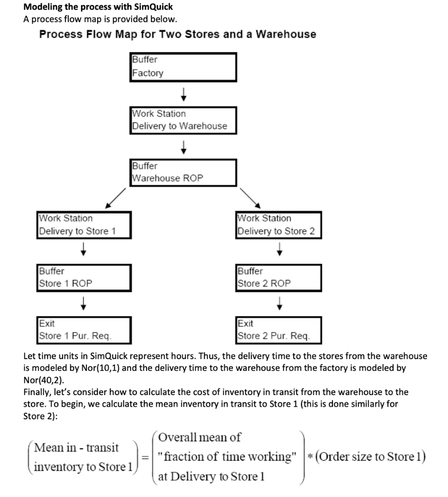
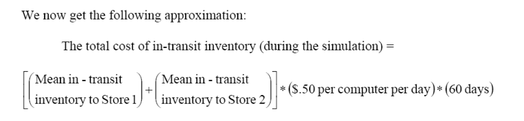
Modeling the process with SimQuick A process flow map is provided below. Process Flow Map for Two Stores and a Warehouse Buffer Factory Work Station Delivery to Warehouse Buffer Warehouse ROP 0-0-0 Work Station Work Station Delivery to Store 2 Buffer Store 2 ROP Exit Store 2 Pur. Req. Let time units in SimQuick represent hours. Thus, the delivery time to the stores from the warehouse is modeled by Nor(10,1) and the delivery time to the warehouse from the factory is modeled by Nor(40,2). Finally, let's consider how to calculate the cost of inventory in transit from the warehouse to the store. To begin, we calculate the mean inventory transit to Store 1 (this is done similarly for Store 2): Overall mean of Mean in - transit inventory to Store 1 "fraction of time working"* (Order size to Store 1) at Delivery to Store 1 Delivery to Store 1 Buffer Store 1 ROP Exit Store 1 Pur. Req. We now get the following approximation: The total cost of in-transit inventory (during the simulation) = Mean in transit Mean in - transit .)]. * ($.50 per computer per day)* (60 days) inventory to Store 1 inventory to Store 2 Warehouse ord. size 100 100 100 200 200 200 Warehouse ROP 50 50 50 50 50 50 Store ord. size 40 45 50 40 45 50 Store ROP 10 10 10 10 10 10 Modeling the process with SimQuick A process flow map is provided below. Process Flow Map for Two Stores and a Warehouse Buffer Factory Work Station Delivery to Warehouse Buffer Warehouse ROP 0-0-0 Work Station Work Station Delivery to Store 2 Buffer Store 2 ROP Exit Store 2 Pur. Req. Let time units in SimQuick represent hours. Thus, the delivery time to the stores from the warehouse is modeled by Nor(10,1) and the delivery time to the warehouse from the factory is modeled by Nor(40,2). Finally, let's consider how to calculate the cost of inventory in transit from the warehouse to the store. To begin, we calculate the mean inventory transit to Store 1 (this is done similarly for Store 2): Overall mean of Mean in - transit inventory to Store 1 "fraction of time working"* (Order size to Store 1) at Delivery to Store 1 Delivery to Store 1 Buffer Store 1 ROP Exit Store 1 Pur. Req. We now get the following approximation: The total cost of in-transit inventory (during the simulation) = Mean in transit Mean in - transit .)]. * ($.50 per computer per day)* (60 days) inventory to Store 1 inventory to Store 2 Warehouse ord. size 100 100 100 200 200 200 Warehouse ROP 50 50 50 50 50 50 Store ord. size 40 45 50 40 45 50 Store ROP 10 10 10 10 10 10